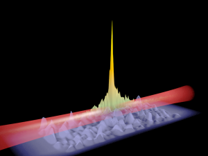
In 1977, the American physicist Philip Warren Anderson received a Nobel Prize in Physics for his discovery of the localization phenomenon in disordered systems, known now as the Anderson localization. This phenomenon is still the subject of many works in Physics and Mathematics, and attracts some famous researchers, such as the Fields Medalist Jean Bourgain. In 2008, the symposium 50 years of Anderson localization was organized at the Institut Henri Poincaré in Paris. You may take a look for instance at the nice article by Lagendijk, van Tiggelen, and Wiersma. Certain mathematical aspects are discussed for instance in an article by Bellissard and the book by Disertori, Kirsch, Klein, Klopp, and Rivasseau.
``Localization [..], very few believed it at the time, and even fewer saw its importance, among those who failed to fully understand it at first was certainly its author. It has yet to receive adequate mathematical treatment, and one has to resort to the indignity of numerical simulations to settle even the simplest questions about it.'' P.W. Anderson, Nobel Lecture, 1977.
Mathematically, the most basic instance of this phenomenon is given by the behavior of the eigenvectors of a one-dimensional discrete Schrödinger operator with a random potential. More precisely, let \(T\) be an \(n\times n\) symmetric tridiagonal matrix with \(T_{i,j}=1\) if \(|i-j|=1\) and \(T_{1,1},\ldots,T_{n,n}\) i.i.d. Bernoulli or Gaussian random variables. It turns out that for a large enough \(n\), with high probability, some of the eigenvectors of \(T\) are heavily localized in space i.e. one of the components of the vector gathers most of the mass of the vector. Probabilistically, the operator \(T\) is close to the random walk in a random potential via a Feynman-Kac formula.
A convenient way to measure the localization of a vector $v\in\mathbb{R}^n$ consists in computing the norm ratio \( r(v):=\left\Vert v\right\Vert_\infty \left\Vert v\right\Vert_2^{-1}\), which takes its values in the interval \( [n^{-1/2},1]\). The more \( r(v)\) is close to \( 1\), the more \(v\) is localized. If \(v\) has unit \( 2\)-norm then localization means a proximity to an extremal point of the \( \ell^1\) unit sphere. In particular, if \( v\) is random and distributed according to the uniform law on the unit sphere, then \( r(v)\) is close to \( n^{-1/2}\) with high probability. This is for instance the case for the rows and columns of random matrices following the Haar distribution on the unitary group. This suggests a transition phenomenon with respect to localization, for random band matrices. Some aspects are considered in e.g. Evers and Mirlin.
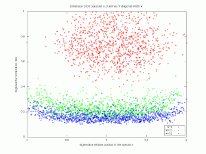
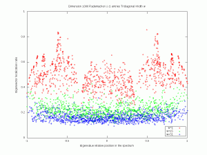
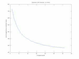
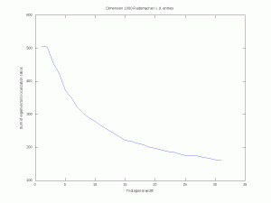
Let us ``resort to the indignity of numerical simulations'' to explore how the band-width of a random band matrix may tune the localization of eigenvectors. For simplicity, we fix \( n=1000\). For \( w\in\{1,\ldots,n-1\}\) we consider the \( n\times n\) symmetric random matrix \( A_w\) with, for all \( 1\leq i\leq j\leq n\), \((A_w)_{i,j}=0\) if \( |i-j|>w\), and where the remaining entries are all i.i.d. standard Gaussian (or symmetric Rademacher). Here are simulations for a single matrix (\( n\) is fixed and \( w\) varies). The localization transition seems to end when \( w\) is near \( \sqrt{n}\approx 32\) and it seems that there is a cutoff in the Rademacher case. A mathematical analysis of eigenvectors localization for random band matrices is considered for instance in a paper by Schenker and a paper by Erdős and Knowles.
Note. The Anderson localization is not a high dimensional phenomenon, and can be checked even on 2x2 matrices. However, the occurence of Anderson localization in high dimensional models is important from the realistic point of view.
Note: we have already explored the localization of eigenvectors of full i.i.d. models in a previous post (and another one). One should not confuse Philip Warren Anderson with Carl David Anderson who received the Nobel Prize in Physics in 1936 for his discovery of the positron and muon.
Notes. From the mathematical point of view, the lack of an exactly solvable model for Anderson localization makes difficult the mathematical analysis of the universality of the phenomenon.
Code: here is the GNU Octave code for the Rademacher case (most of it deals with graphics):
clf; clear; n=1000; dn=1; GFX='gif';
A=diag(sign(randn(1,n))); SumL=[]; LL=[]; SS=[];
for i=1:dn:sqrt(n)
 B=diag(sign(randn(1,n-i)),i);
 A=A+B+B';
 [V,D]=eig(A);
 S=diag(D);
 L=norm(V,Inf,'columns');
 % Save of sum of localizations for curve plot
 SumL=[SumL,sum(L)];
 % Save results for future uses
 LL=[LL,L']; SS=[SS,S];
end %for i
% Plot of curve
clf; plot(SumL,'b-'); hold on;
title(sprintf('Dimension %i Rademacher i.i.d. entries',n));
xlabel('Tridiagonal width');
ylabel('Sum of eigenvectors localization ratios');
print(sprintf(['trirad-curve-%.3d.',GFX],n),['-d',GFX]);
% Plot of three cases
clf; hold on;
N=[1,fix(size(SS,2)/2),size(SS,2)];
C=['r','g','b'];
for i=[1,2,3]
 a=min(SS(:,N(i))); b=max(SS(:,N(i)));
 plot(2*(SS(:,N(i))-(b+a)/2)/(b-a),LL(:,N(i)),[C(i),'o']);
end %for i
title(sprintf(['Dimension %i Rademacher',\
'i.i.d. entries Tridiagonal Width w'],n));
xlabel('Eigenvalue relative position in the spectrum');
ylabel('Eigenvector localization ratio');
legend(sprintf(' w=%i',N(1)),\
sprintf(' w=%i',N(2)),\
sprintf(' w=%i',N(3)),\
"location","southeast");
legend("boxon");
print(sprintf(['trirad-three-%.3d.',GFX],n),['-d',GFX])
5 Comments
