This tiny post is devoted to a phenomenon regarding dilation/truncation/rounding. This can be traced back to Aurel Wintner (1933), P. Kosulajeff (1937), and John Wilder Tukey (1938).
For any real number \( {x} \), let us denote its fractional part by \( {\{ x\}=x-\lfloor x\rfloor\in[0,1)} \).
Note that then \( {\{ 0\}=0} \) while \( {\{ x\}=1-\{|x|\}} \) when \( {x<0} \), thus \( {\{ x\}+\{ -x\}=\mathbf{1}_{x\not\in\mathbb{Z}}} \).
Following Kosulajeff, let \( {X} \) be a real random variable with cumulative distribution function \( {F} \) which is absolutely continuous. Then the fractional part of the dilation of \( {X} \) by a factor \( {\sigma} \) tends in law, as \( {\sigma\rightarrow\infty} \), to the uniform distribution on \( {[0,1]} \). In other words
\[ \{\sigma X\} :=\sigma X-\lfloor \sigma X\rfloor \underset{\sigma\rightarrow\infty}{\overset{\text{law}}{\longrightarrow}}\mathrm{Uniform}([0,1]). \]
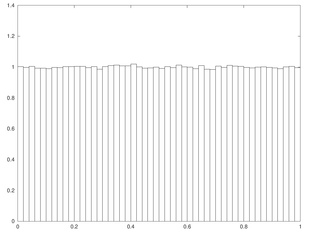
Actually if \( {X\sim\mathcal{N}(0,1)} \) and \( {\sigma=1} \) then \( {\{ X\}} \) is already close to the uniform!
We could find the result intuitive: the law of the dilated random variable \( {\sigma X} \) is close, as the factor \( {\sigma} \) gets large, to the Lebesgue measure on \( {\mathbb{R}} \), and the image measure of it via the canonical projection on \( {[0,1]} \) is uniform. What is unclear is the precise role of local regularity and behavior at infinity of the distribution of \( {X} \).
A proof. Recall that \( {F} \) is absolutely continuous: its derivative \( {F'} \) exists almost everywhere, \( {F'\in\mathrm{L}^1(\mathbb{R},\mathrm{d}x)} \), and \( {F(\beta)-F(\alpha)=\int_\alpha^\beta F'(x)\mathrm{d}x} \) for all \( {\alpha\leq\beta} \). Following Kosulajeff, we start by observing that for every interval \( {[a,b]\subset[0,1)} \),
\[ \begin{array}{rcl} \mathbb{P}(\{\sigma X\}\in [a,b]) &=&\sum_{n\in\mathbb{Z}}\mathbb{P}(\sigma X\in[n+a,n+b])\\ &=&\sum_{n\in\mathbb{Z}}\Bigr(F\Bigr(\frac{n+b}{\sigma}\Bigr)-F\Bigr(\frac{n+a}{\sigma}\Bigr)\Bigr)\\ &=&\sum_{n\in\mathbb{Z}}\int_a^b\frac{1}{\sigma}F'\Bigr(\frac{n+x}{\sigma}\Bigr)\mathrm{d}x. \end{array} \]
Now, if \( {[a,b]} \) and \( {[a',b']} \) are sub-intervals of \( {[0,1)} \) of same length \( {b-a=b'-a'} \),
\[ \int_{a'}^{b'}\frac{1}{\sigma}F'\Bigr(\frac{n+x}{\sigma}\Bigr)\mathrm{d}x =\int_a^{b'-a'+a}\frac{1}{\sigma}F'\Bigr(\frac{n+x-a+a'}{\sigma}\Bigr)\mathrm{d}x =\int_a^{b}\frac{1}{\sigma}F'\Bigr(\frac{n+x-a+a'}{\sigma}\Bigr)\mathrm{d}x, \]
and thus
\[ \begin{array}{rcl} \Bigr| \int_a^b\frac{1}{\sigma}F'\Bigr(\frac{n+x}{\sigma}\Bigr)\mathrm{d}x -\int_{a'}^{b'}\frac{1}{\sigma}F'\Bigr(\frac{n+x}{\sigma}\Bigr)\mathrm{d}x \Bigr| &\leq&\int_a^b\frac{1}{\sigma}\Bigr|F'\Bigr(\frac{n+x}{\sigma}\Bigr)-F'\Bigr(\frac{n+x-a+a'}{\sigma}\Bigr)\Bigr|\mathrm{d}x\\ &=&\int_{\frac{n+a}{\sigma}}^{\frac{n+b}{\sigma}}\Bigr|F'(x)-F'\Bigr(x+\frac{a'-a}{\sigma}\Bigr)\Bigr|\mathrm{d}x. \end{array} \]
Using the fact that the intervals \( {\Bigr[\frac{n+a}{\sigma},\frac{n+b}{\sigma}\Bigr]} \), \( {n\in\mathbb{Z}} \), are pairwise disjoint, we obtain
\[ \begin{array}{rcl} \mathbb{P}(\{\sigma X\}\in [a,b])- \mathbb{P}(\{\sigma X\}\in [a',b']) &\leq& \sum_{n\in\mathbb{Z}}\int_{\frac{n+a}{\sigma}}^{\frac{n+b}{\sigma}}\Bigr|F'(x)-F'\Bigr(x+\frac{a'-a}{\sigma}\Bigr)\Bigr|\mathrm{d}x\\ &\leq&\int_{-\infty}^{+\infty}\Bigr|F'(x)-F'\Bigr(x+\frac{a'-a}{\sigma}\Bigr)\Bigr|\mathrm{d}x\\ &=&\Bigr\|F'-F'\Bigr(\cdot+\frac{a'-a}{\sigma}\Bigr)\Bigr\|_{\mathrm{L}^1(\mathbb{R},\mathrm{d}x)}, \end{array} \]
which goes to zero as \( {\sigma\rightarrow\infty} \) because translations are continuous in \( {\mathrm{L}^1(\mathbb{R},\mathrm{d}x)} \).
Densities. Still following Kosulajeff, if \( {X} \) has a continuous density \( {f} \) with respect to the Lebesgue measure such that \( {f(x)} \) decreases when \( {|x|} \) increases when \( {|x|} \) is large enough, then the density of \( {\{\sigma X\}} \) tends pointwise to \( {1} \) as \( {\sigma\rightarrow\infty} \).
To see it, we start by observing that the density of \( {\{\sigma X\}} \) is
\[ x\in[0,1]\mapsto\sum_{n\in\mathbb{Z}}\frac{1}{\sigma}f\Bigr(\frac{n+x}{\sigma}\Bigr). \]
Let us fix an arbitrary \( {x\in\mathbb{R}} \) and \( {\varepsilon>0} \). Let \( {A>0} \) be large enough such that
\[ \int_{-\sigma A}^{\sigma A}f\Bigr(\frac{y}{\sigma}\Bigr)\mathrm{d}y =\int_{-A}^Af(y)\mathrm{d}y>1-\varepsilon. \]
Now we observe that
\[ \begin{array}{rcl} \Bigr|\sum_{n\in\mathbb{Z}\cap[-\sigma A,\sigma A]}\frac{1}{\sigma}f\Bigr(\frac{n+x}{\sigma}\Bigr)-\int_{-\sigma A}^{\sigma A}\frac{1}{\sigma}f\Bigr(\frac{y}{\sigma}\Bigr)\mathrm{d}y\Bigr| &\leq&\int_{-\sigma A}^{\sigma A}\frac{1}{\sigma}\Bigr|f\Bigr(\frac{\lfloor y\rfloor+x}{\sigma}\Bigr)-f\Bigr(\frac{y}{\sigma}\Bigr)\Bigr|\mathrm{d}y\\ &=&\int_{-A}^{A}\Bigr|f\Bigr(\frac{\lfloor \sigma z\rfloor+x}{\sigma}\Bigr)-f(z)\Bigr|\mathrm{d}z, \end{array} \]
and this last quantity goes to \( {0} \) as \( {\sigma\rightarrow\infty} \) by the uniform continuity of \( {f} \) on \( {[-A,A]} \) which follows from the continuity of \( {f} \) by the Heine theorem. It follows that
\[ \Bigr|\sum_{n\in\mathbb{Z}\cap[-\sigma A,\sigma A]}\frac{1}{\sigma}f\Bigr(\frac{n+x}{\sigma}\Bigr)-1\Bigr|\leq2\varepsilon. \]
On the other hand, since \( {f(x)} \) decreases when \( {|x|} \) increases, for large enough \( {|x|} \), we have, for a large enough \( {A>0} \),
\[ \begin{array}{rcl} \sum_{n\in\mathbb{Z}\cap[-\sigma A,\sigma A]^c}\frac{1}{\sigma}f\Bigr(\frac{n+x}{\sigma}\Bigr) &\leq& \sum_{n\in\mathbb{Z}\cap[-\sigma A,\sigma A]^c}\int_{n-1}^n\frac{1}{\sigma}f\Bigr(\frac{y+x}{\sigma}\Bigr)\mathrm{d}y\\ &\leq&\int_{|y|>\sigma A-1}\frac{1}{\sigma}f\Bigr(\frac{y+x}{\sigma}\Bigr)\mathrm{d}y\\ &=&\int_{|z|>A-\frac{1}{\sigma}}f\Bigr(z+\frac{x}{\sigma}\Bigr)\mathrm{d}z \end{array} \]
which is \( {\leq\varepsilon} \) for \( {A} \) and \( {\sigma} \) large enough. Finally we obtain, as expected,
\[ \Bigr|\sum_{n\in\mathbb{Z}}\frac{1}{\sigma}f\Bigr(\frac{n+x}{\sigma}\Bigr)-1\Bigr|\leq3\varepsilon. \]
Necessary and sufficient condition via Fourier analysis. Following Tukey, for any real random variable \( {X} \), we have that \( {Y=\{\sigma X\}} \) tends in law as \( {\sigma\rightarrow\infty} \) to the uniform law on \( {[0,1]} \) if and only if the Fourier transform or characteristic function \( {\varphi_X} \) of \( {X} \) tends to zero at infinity.
If the cumulative distribution function of \( {X} \) is absolutely continuous then the Riemann-Lebesgue lemma gives that \( {\varphi_X} \) vanishes at infinity, and we recover the result of Kosulajeff. The result of Tukey is however strictly stronger since there exists singular distributions with respect to the Lebesgue measure for which the cumulative distribution function is not absolutely continuous while the Fourier transform vanishes at infinity.
Let us give the proof of Tukey. For every real random variable \( {Z} \) and all \( {t\in\mathbb{R}} \),
\[ \begin{array}{rcl} \varphi_Z(t) &=&\mathbb{E}(\mathrm{e}^{\mathrm{i}tZ})\\ &=&\mathbb{E}(\mathrm{e}^{\mathrm{i}tZ}\sum_{n\in\mathbb{Z}}\mathbf{1}_{Z\in[n,n+1)})\\ &=&\mathbb{E}(\sum_{n\in\mathbb{Z}}\mathrm{e}^{\mathrm{i}t(n+\{ Z\})}\mathbf{1}_{Z\in[n,n+1)}) \\ &=&\mathbb{E}(\mathrm{e}^{\mathrm{i}t\{ Z\}}\sum_{n\in\mathbb{Z}}\mathrm{e}^{\mathrm{i}tn}\mathbf{1}_{Z\in[n,n+1)}). \end{array} \]
But the sum in the right hand side is constant \( {=1} \) if \( {t=2\pi k\in2\pi\mathbb{Z}} \). Hence, with \( {Z=\sigma X} \),
\[ \varphi_{\{\sigma X\}}(2\pi k) =\varphi_{\sigma X}(2\pi k) =\varphi_{X}(2\pi k\sigma), k\in\mathbb{Z}. \]
Therefore \( {\varphi_X} \) vanishes at infinity if and only if
\[ \lim_{\sigma\rightarrow\infty}\varphi_{\{\sigma X\}}(k)=\mathbf{1}_{k\neq0}, k\in\mathbb{Z}. \]
On the other hand, if \( {U} \) is uniformly distributed on \( {[0,1]} \) then for all \( {t\in\mathbb{R}} \),
\[ \varphi_U(t)=\mathbb{E}(\mathrm{e}^{\mathrm{i}tU})=\frac{\mathrm{e}^{\mathrm{i}t}-1}{\mathrm{i}t}\mathbf{1}_{t\neq0}+\mathbf{1}_{t=0} \]
and in particular,
\[ \varphi_U(2\pi k)=\mathbf{1}_{k=0}, k\in\mathbb{Z}. \]
Now, by a Fourier coefficients version of the Paul Lévy theorem, \( {\{\sigma X\}\rightarrow U} \) in law as \( {\sigma\rightarrow\infty} \) if and only if \( {\varphi_{\{\sigma X\}}\rightarrow\varphi_U} \) as \( {\sigma\rightarrow\infty} \) pointwise on \( {2\pi\mathbb{Z}} \). Note that \( {2\pi\mathbb{Z}} \) suffices because the random variables are uniformly bounded. Note also that on a closed interval, for the uniform topology, the trigonometric polynomials are dense in the set of continuous functions.
Regularization by convolution and central limit phenomenon. Suppose that \( {X_1,X_2,\ldots} \) are independent and identically distributed real random variables such that \( {\{kX_1\}} \) is not constant for all \( {k\in\{1,2,\ldots\}} \). Then
\[ \{X_1+\cdots+X_n\} \underset{n\rightarrow\infty}{\overset{\text{law}}{\longrightarrow}}\mathrm{Uniform}([0,1]). \]
To see it, as before, for all \( {k\in\mathbb{Z}} \), \( {\varphi_U(2\pi k)=\mathbf{1}_{k=0}} \) when \( {U\sim\mathrm{Uniform}([0,1])} \), while
\[ \varphi_{\{X_1+\cdots+X_n\}}(2\pi k) =\varphi_{X_1+\cdots+X_n}(2\pi k) =(\varphi_{X_1}(2\pi k))^n \underset{n\rightarrow\infty}{\longrightarrow}\mathbf{1}_{k=0}, \]
since \( {\varphi_{X_1}(0)=1} \) while \( {|\varphi_{X_1}(2\pi k)|<1} \) if \( {k\neq0} \). Indeed for all \( {k} \) the Jensen inequality for the strictly convex function \( {\left|\cdot\right|^2} \) and the complex random variable \( {\mathrm{e}^{\mathrm{i}2\pi kX_1}} \) gives \( {|\varphi_{X_1}(2\pi k)|\leq1} \) with equality if and only if the complex random variable \( {\mathrm{e}^{\mathrm{i}2\pi kX_1}} \) is constant, while for any real random variable \( {Y} \), the following properties are equivalent:
- \( {\mathrm{e}^{\mathrm{i}2\pi Y}} \) is constant;
- \( {Y} \) takes its values in \( {c+\mathbb{Z}} \) for some \( {c\in\mathbb{R}} \);
- \( {\{Y\}} \) is constant.
Note that \( {\{X_1+\cdots+X_n\}=\{X_1\}+\cdots+\{X_n\}} \) where the additions in the right hand side take place in the quotient space \( {\mathbb{R}/[0,1]=\mathbb{S}^1} \), which is a compact Lie group. Actually the statement that we have obtained can be seen as a Central Limit Theorem on a compact Lie group, for which the uniform distribution plays the role of the Gaussian. There is no need for a dilation factor thanks to compactness. Note that the central limit phenomenon states that \( {X_1+\cdots+X_n} \) is close to \( {\mathcal{N}(nm,n\sigma^2)} \) as \( {n} \) is large, where \( {m} \) and \( {\sigma^2} \) are the mean and variance of the \( {X_i} \)'s. Note also that taking the fractional part corresponds to project \( {\mathbb{R}} \) on the unit circle \( {\mathbb{S}^1=\mathbb{R}/[0,1]} \) by using the canonical projection. This leads to a general notion of CLT on Lie groups which can be studied using Fourier analysis.
Rounding. The rounding of \( {x} \) takes the form \( {\sigma^{-1}\lfloor\sigma x\rfloor} \), and the Wintner-Kosulajeff-Tukey phenomenon states that the rounding error \( {x-\sigma^{-1}\lfloor\sigma x\rfloor} \) becomes uniform as \( {\sigma\rightarrow\infty} \).
Fractional part. Beware that \( {\{ 1.3\}=0.3} \) while \( {\{ -1.3\}=0.7} \). It could be possible to use the following alternative notion of fractional part: \( {\langle x\rangle=x-\lfloor x\rfloor=\{x\}} \) if \( {x\geq0} \) and \( {\langle x\rangle=x-\lceil x\rceil=1-\{x\}} \) if \( {x<0} \), which gives \( {\langle -1.3\rangle=0.3} \). However, the asymptotic results of this post for \( {\{\cdot\}} \) remain valid for \( {\langle\cdot\rangle} \) since the map \( {x\in[0,1]\mapsto1-x} \) leaves invariant the uniform distribution on \( {[0,1]} \).
Weyl equipartition theorem. The Weyl equipartition theorem in analytic number theory is a sort of deterministic version. More precisely, a real sequence \( {{(x_n)}_n} \) is uniformly distributed modulo \( {1} \) in the sense of Weyl when for any Borel subset \( {I\subset [0,1]} \) of Lebesgue measure \( {|I|} \),
\[ \lim_{n\rightarrow\infty}\frac{\mathrm{Card}\{k\in\{1,\ldots,n\}:\{ x_k\}\in I\}}{n}=|I|. \]
Now the famous equipartition or equidistribution theorem proved by Hermann Weyl in 1916 states that this is equivalent to say that for all \( {m\in\mathbb{Z}} \), \( {m\neq0} \),
\[ \lim_{n\rightarrow\infty}\frac{1}{n}\sum_{k=1}^n\mathrm{e}^{2\pi\mathrm{i}mx_k}=0. \]
A proof may consist in approximating the indicator of \( {I} \) by trigonometric polynomials.
Jacobi theta function. In the special case \( {X\sim\mathcal{N}(0,1)} \) the density of \( {\{\sigma X\}} \) at point \( {x\in[0,1]} \) is given by
\[ \frac{1}{\sqrt{2\pi}\sigma} \sum_{n\in\mathbb{Z}}\mathrm{e}^{-\frac{(n+x)^2}{2\sigma^2}} =\frac{\mathrm{e}^{-\frac{x^2}{2\sigma^2}}}{\sqrt{2\pi}\sigma} \sum_{n\in\mathbb{Z}}\mathrm{e}^{-\frac{n^2}{2\sigma^2}+\frac{nx}{\sigma^2}} =\frac{\mathrm{e}^{-\frac{x^2}{2\sigma^2}}}{\sqrt{2\pi}\sigma} \vartheta(-\mathrm{i}/(2\pi\sigma^2),\mathrm{i}/(2\pi\sigma^2)) \]
where
\[ \vartheta(z,\tau) =\sum_{n\in\mathbb{Z}} \mathrm{e}^{\pi\mathrm{i}n^2\tau+2\pi\mathrm{i}nz} =\sum_{n\in\mathbb{Z}}(\mathrm{e}^{\pi\mathrm{i}\tau})^{n^2}\cos(2\pi nz) \]
is the Jacobi theta function, as special function that plays a role in analytic number theory. Note that the Greek letter \( {\vartheta} \) is a variant of \( {\theta} \), obtained in LaTeX with the command vartheta.
This is the path followed by Wintner, in relation with a rather sketchy Fourier analysis. Actually the main subject of the 1933 paper by Wintner was to show that the Gaussian law is the unique stable distribution with finite variance. His analysis led him at the end of his short paper to consider another problem: the uniformization of the fractional part of a Gaussian with a blowing variance! Wintner was fond of probability theory and number theory.
About Kosulajeff. Kosulajeff cites Wintner, and is cited by Tukey. It seems that P. Kosulajeff, also written P. A. Kozulyaev, or Petr Alekseevich Ozulyaev, was a former doctoral student of Andrey Kolmogorov, who saved him from the Staline great purge. This information comes from Laurent Mazliak (via my friend Arnaud Guyader), who reads Russian and knows the history of probability.
Personal. I have encountered this phenomenon fifteen years ago while working on a statistical problem with my colleague Didier Concordet. At that time, I was not aware of the literature so I had to rediscover everything in particular the role of absolute continuity. Fun! Recently, by accident, I have encoutered again this striking phenomenon in relation with a research project for master students about a Monte Carlo algorithm for stochastic billiards. I have discussed a little bit the problem with my colleague Marc Hoffmann, who also knew this phenomenon from the community of the general theory of stochastic processes and mathematical finance.
Bibliography.
- Aurel Wintner, On the Stable Distribution Laws, American Journal of Mathematics, Vol. 55, No. 1 (1933), pp. 335-339.
- P. Kosulajeff, Sur la répartition de la partie fractionnaire d'une variable, Rec. Math. [Mat. Sbornik] N.S., 1937, Volume 2(44), Number 5, 1017-1019
- John Wilder Tukey, On the distribution of the fractional part of a statistical variable, Rec. Math. [Mat. Sbornik] N.S., 1938, Volume 4(46), Number 3, 561-562
- Sylvain Delattre and Jean Jacod, A central limit theorem for normalized functions of the increments of a diffusion process, in the presence of round-off errors, Bernoulli Volume 3, Number 1 (1997), 1-28.
- Pierre-Henri Cumenge, P-variations approchées et erreurs d'arrondis, thèse de doctorat sous la direction de Jean Jacod, soutenue en 2011.
- Vladimír Holý, How big is the rounding error in financial high-frequency data? AIP Conference Proceedings 1978, 470076 (2018)
- David Applebaum, Probability on Compact Lie Groups, Probability Theory and Stochastic Modelling 70, Springer, 2014. xxvi+217 pp.
- Bakir Farhi, Sur l’ensemble exceptionnel de Weyl (About the Weyl’s exceptional set), C. R. Acad. Sci. Paris, Sér. I 343 (2006), p. 441-445.
- Hermann Weyl, Über die Gleichverteilung von Zahlen mod Eins. Math. Ann, 77 (1916), p. 313-352.
f(x) grows with |x| ? I would say the contrary…
And for « fifty years ago », I do not believe you 😉
🙂 Thanks Amic! Fixed.