This tiny post is about the ubiquity of Gaussian distributions. Here are three reasons.
Geometry. A random vector of dimension two or more has independent components and is rotationally invariant if and only if its components are Gaussian, centered, with same variances.
In other words, for all $n\geq2$, a probability measure on $\mathbb{R}^n$ is in the same time product and spherically symmetric if and only if it is a Gaussian law $\mathcal{N}(0,\sigma^2I_n)$ for some $\sigma\geq0$.
Note that this does not work for $n=1$. In a sense it is a purely multivariate phenomenon. It is remarkable that the statement does not involve any condition on moments or integrability.
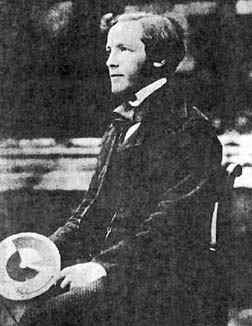
This observation goes back at least to James Clerk Maxwell (1831 - 1879) in physics and kinetic theory. Such a characterization by mean of invariance by a group of transformations is typical of geometry or in a sense Felix Klein algebraization of geometry. A matrix version of this phenomenon provides a characterization of Gaussian ensembles of random matrices by mean of unitary invariance and independence of the entries. More can be found in a previous post.
Optimization. Among the probability measures with fixed variance and finite entropy, the maximum entropy is reached by Gaussian distributions. In other words, if we denote by $S(f)=-\int f(x)\log(f(x))\mathrm{d}x$ the entropy of a density $f:\mathbb{R}^n\to\mathbb{R}_+$, and if \[\int V(x)f(x)\mathrm{d}x=\int V(x)f_\beta(x)\mathrm{d}x\quad\mbox{with}\quad f_\beta(x)=\frac{\mathrm{e}^{-\beta V(x)}}{Z_\beta}\mbox{ and }V(x)=|x|^2\] then the Jensen inequality for the strictly convex function $u\geq0\mapsto u\log(u)$ gives \[\mathcal{S}(f_\beta) - \mathcal{S}(f) =\int\frac{f}{f_\beta}\log\frac{f}{f_\beta}f_\beta\mathrm{d}x \geq\left(\int\frac{f}{f_\beta}f_\beta\mathrm{d}x\right)\log\left(\int\frac{f}{f_\beta}f_\beta\mathrm{d}x\right)=0,\] with equality if and only if $f=f_\beta$. This works beyond Gaussians for non-quadratic $V$'s.
This observation goes back at least to Ludwig Boltzmann (1844 - 1906) in kinetic theory. Nowadays it is an essential fact for statistical physics, statistical mechanics, and Bayesian statistics. More can be found in a previous post see also this one.
Probability. The univariate Gaussian distribution is the unique stable distribution with finite variance. In other words if $X$ is a real random variable with finite variance such that every linear combination of independent copies of it is distributed as a dilation of it, then it is Gaussian.$$\mathrm{Law}(a_1X_1+\cdots+a_nX_n)=\mathrm{Law}\Bigr(\sqrt{a_1^2+\cdots+a_n^2}X\Bigr).$$ As a consequence of this stability by convolution, if we sum up $n$ independent copies of a square integrable random variable and scale the sum by $\sqrt{n}$ to fix the variance, then the limit as $n\to\infty$ can only be Gaussian. This is the central limit phenomenon. This observation goes back, in a combinatorial simple form, at least to Abraham de Moivre (1667 - 1754) via\[\binom{n}{k}p^k(1-p)^{n-k} \simeq \frac{1}{\sqrt{2 \pi np(1-p)}}\mathrm{e}^{-\frac{(k-np)^2}{2np(1-p)}}.\] A more general version states that if $X_1,\ldots,X_n$ are independent centered random vectors of $\mathbb{R}^d$ with same covariance matrix $\Sigma$, the increments of a random walk, then $$\mathrm{Law}\Bigr(\frac{X_1+\cdots+X_n}{\sqrt{n}}\Bigr)\underset{n\to\infty}{\longrightarrow}\mathcal{N}(0,\Sigma).$$ The phenomenon holds as soon as the variance of the sum is well spread among the elements of the sum in order to get stability by convolution. More can be found in a previous post.
Note that the discrete time is at the order of the squared space. A time-space scaling leads, from random walks, via the central limit phenomenon, to Brownian motion and the heat equation$$\partial_t p(t,x)=\Delta_x p(t,x)\quad\mbox{where}\quad p(t,x)=(4\pi t)^{-\frac{d}{2}}\mathrm{e}^{-\frac{|x|^2}{4t}}.$$ The Laplacian differential operator appears in this scaling limit via a second order Taylor expansion as the infinitesimal effect of the increments, and has the invariances of the Gaussian.
Actually the Gaussian density is invariant by the Fourier transform in the sense that $$(2\pi)^{-\frac{d}{2}}\int_{\mathbb{R}^d}\mathrm{e}^{-\frac{|x|^2}{2}}\mathrm{e}^{\mathrm{i}\langle \theta,x\rangle}\mathrm{d}x=\mathrm{e}^{-\frac{|\theta|^2}{2}},$$and this allows to solve the heat equation as observed by Joseph Fourier (1768 -- 1830). The Fourier transform is also useful for the analysis of the stability by convolution, the central limit phenomenon, and Brownian motion, as observed by Paul Lévy (1886 -- 1971).
There are multiple links between all these aspects. For instance the Boltzmann observation is related to the Boltzmann equation, to the Maxwell observation, and to the heat equation.
The standard Gaussian distribution is also characterized by the Gaussian integration by parts which states that $X\sim\mathcal{N}(0,1)$ if and only if for any slowly growing test function $f:\mathbb{R}\to\mathbb{R}$,
$$
\mathbb{E}(Xf(X))=\mathbb{E}(f'(X)).
$$
The specialization to $f(x)=x^n$ leads to the combinatorial characterization of the standard Gaussian distribution by the moments recursion: $\mathbb{E}(X^{n+1})=n\mathbb{E}(X^{n-1})$. The Gaussian integration by parts is at the heart of the Stein method for proving central limit theorems, and also at the heart of the Malliavin calculus, developped at the origin to provide a probabilistic alternative to the Fourier approach for the Hörmander theorem on hypoelliptic operators.
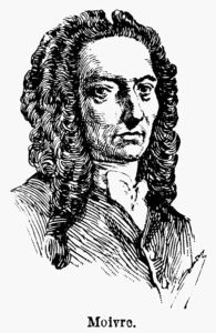
(1667 - 1754)
J'aurais quand meme dit une quatrieme raison avec l'equation de la chaleur... decouverte par fourier ou un autre d'ailleurs (ma memoire flanche) et sans lien initial avec le TCL...
Salut Arnaud. Tu ne ferais pas des probas liées aux ÉDP, toi ? 😉 À l'origine il y avait effectivement un quatrième item consacré à la transformée de Fourier ! Concernant l'équation de la chaleur, c'est bien entendu une raison historique importante, mais sur le fond, avec le recul, on sait aujourd'hui qu'elle n'est que la limite d'échelle des marches aléatoires via le TLC, comme évoqué à la fin... C'est le même bloc en quelque sorte. J'en ai rajouté quand même un peu plus avec Fourier et Lévy notamment. Il y a aussi le lien avec l'isopérimétrie sur la sphère, mais cela semble anecdotique en comparaison du reste, et à nouveau relié au TLC ! Tout cela étant dit, ce billet n'a pas pour but ni prétention de faire un historique de la gaussienne à travers le temps, mais plutôt de lister quelques raisons profondes de son ubiquité, et de mentionner des (plutôt que « les ») sources historiques associées. En particulier, rien n'est dit sur Gauss, un comble !