Gumbel fit with Julia

The Gumbel distribution appears in the modelling of extreme values phenomena and the famous Fisher–Tippett–Gnedenko theorem. Its cumulative distribution function is given by

$$x\in\mathbb{R}\mapsto\exp\left(-\exp\left(-\frac{x-\mu}{\sigma}\right)\right)$$

where $\mu\in\mathbb{R}$ and $\sigma\in(0,\infty)$ are location and scale parameters. Its mean and variance are

$$\mu+\gamma\sigma\quad\text{and}\quad\frac{\pi^2\sigma^2}{6},$$

where $\gamma=0.577\ldots$ is Euler’s constant. The maximum likelihood estimators $\hat{\mu}$ and $\hat{\sigma}$ satisfy

$$
\hat{\mu} =-\hat{\sigma}\log\left(\frac{1}{n}\sum_{i=1}^{n}\mathrm{e}^{-x_i/\hat{\sigma}}\right)\quad\text{and}\quad\hat{\sigma} = \frac{\sum_{i=1}^nx_i}{n}-\frac{\sum_{i=1}^{n} x_i\mathrm{e}^{-x_i/\hat{\sigma}}}{ \sum_{i=1}^{n} \mathrm{e}^{-x_i/\hat{\sigma}}}.
$$

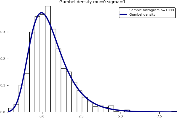
Note that the second formula is implicit. Unfortunately, the current version of the Julia package Distributions.jl does not implement yet the Gumbel distro in fit()/fit_mle(). Here is a home brewed program to fit a Gumbel distribution on data using maximum likelihood and moments. The produced graphic is above. Note that the GNU R software implements a Gumbel fit in the fitdistrplus package with a notable contribution from my colleague Christophe Dutang.

# Pkg.add("Roots") # https://github.com/JuliaMath/Roots.jl
using Roots
""" 
Computes approximately the Maximum Likelihood Estimator (MLE) of 
the position and scale parameters of a Gumbel distribution with
cumulative distribution function x-> exp(-exp(-(x-mu)/sigma)).
Has mean mu+eulergamma*sigma and variance sigma^2*pi^2/6.
The MLE for mu is a function of data and the MLE for sigma.
The MLE for sigma is the root of a nonlinear function of data,
computed numerically with function fzero() from package Roots.

Reference: page 24 of book ISBN 1-86094-224-5.
Samuel Kotz and Saralees Nadarajah
Extreme value distributions.Theory and applications. 
Imperial College Press, London, 2000. viii+187 pp. 
https://ams.org/mathscinet-getitem?mr=1892574 

``no distribution should be stated without an explanation of how the
parameters are estimated even at the risk that the methods used will 
not stand up to the present rigorous requirements of mathematically 
minded statisticians''. E. J. Gumbel (1958).
"""
function gumbel_fit(data)
  f(x) = x - mean(data) + sum(data.*exp(-data/x)) / sum(exp(-data/x)) 
  sigma = fzero(f,sqrt(6)*std(data)/pi) # moment estimator as initial value
  mu = - sigma * log(sum(exp(-data/sigma))/length(data))
  return mu , sigma
end #function

# Pkg.add("Plots") # https://github.com/JuliaPlots/Plots.jl
# Pkg.add("PyPlot") # https://github.com/JuliaPy/PyPlot.jl
# http://docs.juliaplots.org/
using Plots
function gumbel_fit_plots(data,label,filename) 
  n = length(data)
  data = reshape(data,n,1)
  mu , sigma = gumbel_fit(data)
  X = collect(linspace(minimum(data),maximum(data),1000))
  tmp = (X-mu)/sigma
  Y = exp(-tmp-exp(-tmp))/sigma
  pyplot()
  histogram!(data,
             nbins = round(Int,sqrt(n)),
             normed = true,
             label = @sprintf("%s histogram n=%i",label,n),
             color = :white)
  plot!(X,Y,
        title = @sprintf("Gumbel density mu=%2.2f sigma=%2.2f",mu,sigma),
        titlefont = font("Times", 10),
        label = "Gumbel density",
        lw = 3,
        linestyle = :solid, 
        linecolor = :darkblue,
        grid = false,
        border = false)
        gui()
  #savefig(string(filename,".svg"))
  savefig(string(filename,".png"))
end #function

function gumbel_fit_example()
  gumbel_fit_plots(-log(-log(rand(1,1000))),"Sample","gumbelfitexample") 
end #function