This short post is about a joint work with François Bolley and Joaquín Fontbona on a Dyson Ornstein-Uhlenbeck process, published a few years ago. The numerics and graphics are new.
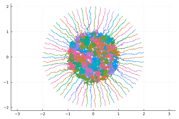
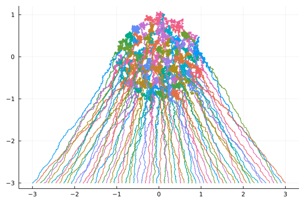

Above, two numerical experiments with $N=66$ particles and initial conditions on a uniform grid on a circle, and on a segment. Data is displayed as moving particles as well as trajectories. The one started from a segment is run ten times slower than the one started from a circle. These interacting particles on $\mathbb{R}^2=\mathbb{C}$ follow the Dyson Ornstein-Uhlenbeck dynamics
$$
\mathbb{d}X^{i,N}_t
=\sqrt{\frac{2}{N}}\mathbb{d} B^{i,N}_t
-2X^{i,N}_t\,\mathbb{d} t
-\frac{\beta}{N}\sum_{j\neq i}\frac{X^{j,N}_t-X^{i,N}_t}{|X^{i,N}_t-X^{j,N}_t|^2}\mathbb{d}t,
\quad 1\leq i\leq N,
$$
where $\beta\geq0$ is a parameter and $B$ is a standard Brownian motion on $(\mathbb{R}^2)^N=\mathbb{C}^N$.
The long time behavior of the particle system is
$$
X^N_t
\overset{\mathrm{law}}{\underset{t\to\infty}{\longrightarrow}}
X^N_\infty
$$
where $X^N_\infty$ follows the $\beta$ Ginibre planar Coulomb gas
$$
\frac{\mathrm{e}^{-N\sum_{i=1}^N|x_i|^2}}{Z_N}
\prod_{1\leq i < j\leq N}|x_i-x_j|^\beta
\mathrm{d}x_1\cdots\mathrm{d}x_N,
$$
while the high dimensional limit at equilibrium is the uniform law on a disc
$$
\frac{1}{N}\sum_{i=1}^N\delta_{X^{i,N}_\infty}
\overset{\mathrm{weak}}{\underset{N\to\infty}{\longrightarrow}}
\frac{\mathbf{1}_{z\in\mathbb{C}:|z|\leq\sqrt{\frac{\beta}{2}}}}{\pi}.
$$
Barycenter (first moment) of the cloud of particles. The stochastic process ${(m_t)}_{t\geq0}={(\frac{1}{N}\sum_{i=1}^nX^{i,N}_t)}_{t\geq0}$ is an Orsntein-Uhlenbeck process solving
$$
\mathrm{d}m_t=\sqrt{\frac{2}{N^2}}\mathrm{d}W_t-2m_t\mathrm{d}t
$$
where $W$ is a standard Brownian motion on $\mathbb{R}^2=\mathbb{C}$. In particular, for $t\geq0$,
$$
m_t\sim\mathcal{N}\Bigr(m_0\mathrm{e}^{-2t},\frac{1-\mathrm{e}^{-4t}}{2N^2}I_2\Bigr).
$$
This follows from the Itô formula and the fact that the real and imaginary parts of the first moment are eigenfunctions of the Dyson Ornstein-Uhlenbeck operator.
Second moment of the cloud of particles. The process ${(R_t)}_{t\geq0}={(\frac{1}{N}\sum_{i=1}^n|X^{i,N}_t|^2)}_{t\geq0}$ is a Cox-Ingersoll-Ross process ${(R_t)}_{t\geq0}$ solving the stochastic differential equation
$$
\mathrm{d}R_t = \sqrt{\frac{8}{N^2}R_t}\mathrm{d}W_t
+4\left[\frac{1}{N}+ \frac{\beta}{4}\frac{N-1}{N}-R_t \right]\mathrm{d}t,
$$
where ${(W_t)}_{t\geq0}$ is a real standard Brownian motion. In particular, its invariant distribution is the Gamma law $\Gamma_N=\mathrm{Gamma}(a,\lambda)$ with shape parameter $a=N+\frac{\beta}{4}N(N-1)$ and scale parameter $\lambda=N^2$. Moreover, for any initial condition $R_0$ and $t \geq 0$,
$$
\begin{align*}
\mathrm{Wasserstein}_1(\mathrm{Law}(R_t),\Gamma_N)
&\leq \mathrm{e}^{-4t}\mathrm{Wasserstein}_1(\mathrm{Law}(R_0),\Gamma_N)\\
\mathbb{E}[R_t\mid R_0]
&= R_0\mathrm{e}^{-4t}+\Bigr(\frac{1}{N}+\frac{\beta}{4}\frac{N-1}{N}\Bigr)(1-\mathrm{e}^{-4t}).
\end{align*}
$$
Note that $\frac{\beta}{4}$ is the second moment of the uniform distribution on the disc of radius $\sqrt{\frac{\beta}{2}}$.
This follows from Itô's formula, Lévy's characterization of BM, and the fact that the second moment is, up to a constant, an eigenfunction of the Dyson Ornstein-Uhlenbeck operator.
Open problem. Compute the spectral gap of the dynamics, or find how it depends over $N$.
Julia code.
using Plots

# Define the 2D Dyson Ornstein-Uhlenbeck process
Base.@kwdef mutable struct DOU2D
    n::Int = 2         # number of particles
    β::Float64 = 2.    # repulsion parameter
    T::Float64 = 10.   # terminal time
    dt::Float64 = 1E-3 # time increment
    r::Float64  = 1.   # initial conditions uniform on segment [-r,r]+3*im
    m = floor(Int, T / dt) # number of times
    x::Array{Complex{Float64},2} = zeros(Complex{Float64},m,n)
end # end struct

function compute!(X::DOU2D)
    # initial condition on grid on centered circle of radius r
    #Theta = range(1, X.n, length = X.n) * 2 * pi / X.n
    #X.x[1,:] = X.r * (cos.(Theta) + im * sin.(Theta)) # unif grid on circle
    # initial condition on grid on segment [-r,r] - 3*im
    X.x[1,:] = range(-X.r, X.r, length = X.n) .- 3 * im
    # trajectories
    for i = 2:X.m
     dB = (randn(1,X.n) + im * randn(1,X.n))/sqrt(2)
     X.x[i,:] = copy(X.x[i-1,:])
     for j in 1:X.n # particles
         X.x[i,j] += sqrt(2/X.n) * dB[j] * sqrt(X.dt)
         X.x[i,j] += -2 * X.x[i-1,j] * X.dt
         for k in 1:X.n
             if (j == k) continue end
             X.x[i,j] += X.β * X.dt / (X.n * (conj(X.x[i-1,j] - X.x[i-1,k])))
         end # for
     end # for
    end # for
end # function

# process and graphics
dou = DOU2D(n = 66, r = 3., T = 5., dt = 1E-4)
compute!(dou)
#
pdou2d = plot()
for j in 1:dou.n # particles
    plot!(pdou2d, real(dou.x[:,j]), imag(dou.x[:,j]), aspect_ratio =:equal, legend = false)
end # for
savefig(pdou2d,"dou2d.png")
savefig(pdou2d,"dou2d.svg")
#
r = dou.r + 1
anim = @animate for i = 1:100:dou.m
    scatter(real(dou.x[i,:]), imag(dou.x[i,:]),
            xlims = (-r,r), ylims = (-r,r),
            aspect_ratio =:equal, legend = false)
end
gif(anim, "dou2danim.gif", fps = 10)
Further reading.
- François Bolley, Djalil Chafaï, and Joaquín Fontbona
Dynamics of a planar Coulomb gas
Annals of Applied Probability 28(5) 3152-3183 (2018) - Djalil Chafaï and Grégoire Ferré
Simulating Coulomb gases and log-gases with hybrid Monte Carlo algorithms
Journal of Statistical Physics 174(3):692-714 (2019) - Yulong Lu and Jonathan C. Mattingly
Geometric ergodicity of Langevin dynamics with Coulomb interactions
Nonlinearity 33(2) 675-699 (2020)