
This short post is devoted to a couple of Julia programs.
Gaussian Unitary Ensemble. It is the Boltzmann-Gibbs measure with density proportional to
$$
(x_1,\ldots,x_N)\in\mathbb{R}^N\mapsto\mathrm{e}^{-N\sum_{i=1}^N x_i^2}\prod_{i<j}(x_i-x_j)^2.
$$
It is the distribution of the eigenvalues of a random $N\times N$ Hermitian matrix distributed according to the Gaussian probability measure with density proportional to
$$
H\mapsto\mathrm{e}^{-N\mathrm{Tr}(H^2)}.
$$
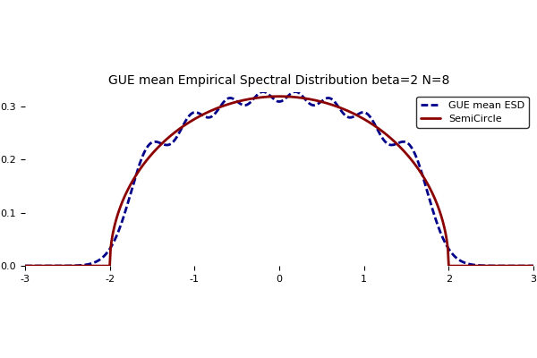
It is a famous exactly solvable model of mathematical physics. There is a nice formula for the mean empirical spectral distribution $\mathbb{E}\mu_N$ where $\mu_N=\frac{1}{N}\sum_{i=1}^N\delta_{x_i}$, namely
$$
x\in\mathrm{R}\mapsto\frac{\mathrm{e}^{-\frac{N}{2}x^2}}{\sqrt{2\pi N}}\sum_{\ell=0}^{N-1}P_\ell^2(\sqrt{N}x)
$$
where ${(P_\ell)}_{\ell\geq0}$ are the Hermite polynomials which are the orthonormal polynomials for the standard Gaussian distribution $\mathcal{N}(0,1)$. The computation of the Laplace transform and a subtle reasonning, see this paper, reveal that it converges as $N\to\infty$ towards the the Wigner semicircle distribution with density with respect to the Lebesgue measure
$$
x\in\mathbb{R}\mapsto\frac{\sqrt{4-x^2}}{2\pi}\mathbf{1}_{x\in[-2,2]}.
$$
Here is a nice plot followed by the Julia code used to produce it.
function normalized_hermite_polynomials_numeric(n,x)
    if size(x,2) != 1
        error("Second argument must be column vector.")
    elseif n == 0
        return ones(length(x),1)
    elseif n == 1
        return x
    else
        P = [ ones(length(x),1) x ]
        for k = 1:n-1
            P = [ P  x.*P[:,k+1]/sqrt(k+1)-P[:,k]*sqrt(1/(1+1/k)) ]
        end
        return P # matrix with columns P_0(x),...,P_n(x)
    end
end #function

function gue_numeric(n,x)
    if size(x,2) != 1
        error("Second argument must be column vector.")
    else
        y = sqrt(n)*x
        p = normalized_hermite_polynomials_numeric(n-1,y).^2
        return exp(-y.^2/2) .* sum(p,2) / sqrt(2*pi*n)
    end
end #function

# Pkg.add("Plots") # http://docs.juliaplots.org/latest/tutorial/
using Plots
pyplot()
N = 8
X = collect(-3:.01:3)
Y = gue_numeric(N,X)
function semicircle(x)
    if (abs(x)>2) return 0 else return sqrt(4-x^2)/(2*pi) end
end # function
Y = [Y [semicircle(x) for x in X]]
plot(X,Y,
     title = @sprintf("GUE mean Empirical Spectral Distribution beta=2 N=%i",N),
     titlefont = font("Times", 10),
     label = ["GUE mean ESD" "SemiCircle"],
     lw = 2,
     linestyle = [:dash :solid],
     linecolor = [:darkblue :darkred],
     aspect_ratio = 2*pi,
     grid = false,
     border = false)
gui()
#savefig("gue.svg")
savefig("gue.png")
Here is, just for fun, a way to produce symbolically Hermite polynomials.
# Pkg.add("Polynomials") # http://juliamath.github.io/Polynomials.jl/latest/
using Polynomials

function unnormalized_hermite_polynomial_symbolic(n)
    if n == 0
        return Poly([1])
    elseif n == 1
        return Poly([0,1])
    else
        P = [Poly([1]) Poly([0,1])]
        for k = 1:n-1
            P = [ P Poly([0,1])*P[k+1]-k*P[k] ]
        end
        return P # better than just P[n+1]
    end
end #function
Complex Ginibre Ensemble. It is the Boltzmann-Gibbs measure with density proportional to
$$
(x_1,\ldots,x_N)\in\mathbb{C}^N\mapsto\mathrm{e}^{-N\sum_{i=1}^N|x_i|^2}\prod_{i<j}|x_i-x_j|^2.
$$
It is the distribution of the eigenvalues of a random $N\times N$ complex matrix distributed according to the Gaussian probability measure with density proportional to
$$
M\mapsto\mathrm{e}^{-N\mathrm{Tr}(MM^*)}
$$
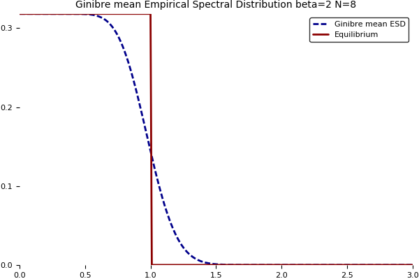
where $M^*=\overline{M}^\top$. Yet another exactly solvable model of mathematical physics, with a nice formula for the mean empirical spectral distribution $\mathbb{E}\mu_N$ where $\mu_N=\frac{1}{N}\sum_{i=1}^N\delta_{x_i}$, given by
$$
z\in\mathbb{C}\mapsto\frac{\mathrm{e}^{-N|z|^2}}{\pi}\sum_{\ell=0}^{N-1}\frac{|\sqrt{N}z|^{2\ell}}{\ell!}
$$
which is the analogue of the one given above for the Gaussian Unitary Ensemble. Using induction and integration by parts, it turns out that this density can be rewritten as
$$
z\in\mathbb{C}\mapsto\int_{N|z|^2}^\infty\frac{u^{N-1}\mathrm{e}^{-u}}{\pi(N-1)!}\mathrm{d}u
=\frac{\Gamma(N,N|z|^2)}{\pi}
$$
where $\Gamma$ is the normalized incomplete Gamma function and where we used the identity
$$
\mathrm{e}^{-r}\sum_{\ell=0}^n\frac{r^\ell}{\ell!}=\frac{1}{n!}\int_r^\infty u^n\mathrm{e}^{-u}\mathrm{d}u.
$$
Note that the function $t\mapsto 1-\Gamma(N,t)$ is the cumulative distribution function of the Gamma distribution with shape parameter $N$ and scale parameter $1$. As a consequence, denoting $X_1,\ldots,X_N$ i.i.d. exponential random variables of unit mean, the density can be written as
$$
z\in\mathbb{C}\mapsto\frac{1}{\pi}\mathbb{P}\left(\frac{X_1+\cdots+X_N}{N}\geq|z|^2\right).
$$
Now the law of large numbers implies that this density converges pointwise as $N\to\infty$ towards the density of the uniform distribution on the unit disk of the complex plane
$$
z\in\mathbb{C}\mapsto\frac{\mathbf{1}_{|z|\leq1}}{\pi}.
$$
One can also use i.i.d. Poisson random variables $Y_1,\ldots,Y_N$ of mean $|z|^2$, giving
$$
z\in\mathbb{C}\mapsto\frac{1}{\pi}\mathbb{P}\left(\frac{Y_1+\cdots+Y_N}{N}<1\right),
$$
see this former post. Here are the plots with respect to $|z|$, followed by the Julia code.
# Pkg.add("Distributions") # https://juliastats.github.io/Distributions.jl
# Pkg.add("Plots") # http://docs.juliaplots.org/latest/tutorial/
using Plots
using Distributions
N = 8
X = collect(0:.01:3)
Y = ccdf(Gamma(N,1),N*X.^2)/pi
function unit(x)
    if (x>1) return 0 else return 1/pi end
end # function
Y = [Y [unit(x) for x in X]]
pyplot()
plot(X,Y,
     title = @sprintf("Ginibre mean Empirical Spectral Distribution beta=2 N=%i",N),
     titlefont = font("Times", 10),
     label = ["Ginibre mean ESD" "Equilibrium"],
     lw = 2,
     linestyle = [:dash :solid],
     linecolor = [:darkblue :darkred],
     grid = false,
     border = false)
gui()
#savefig("ginibre.svg")
savefig("ginibre.png")
Further reading. The Introducing Julia wikibook on Wikibooks.