Have you ever opened The Oxford Handbook of Random Matrix Theory edited by Akemann, Baik, and Di Francesco? The short foreword by Freeman Dyson is fun. I was intrigued, page 16, by a sentence in chapter 2 ("History - An overview", by Bohigas and Weidenmüller):
... That search and, as he says (see page 225 of Ref. [Por65]), the 'accidental' discovery of the Wishart ensemble of random matrices in an early version of the book by Wilks [Wil62], motivated Wigner to use random matrices.
I already knew Wilks's book [Wil62], but not [Por65], which turned out to be a book:
Statistical Theories of Spectra: Fluctuations, A Collection of Reprints and Original Papers. With an introductory Review by Charles E. Porter, Brookhaven National Laboratory, New York. Academic Press, 1965.
I've bought a used copy of this book. Wigner's paper is a conference proceedings p. 223-225:
Proceedings of the International Conference on the Neutron Interactions with the Nucleus. Held at Columbia University, New York, September 9-13, 1957. Published by the United States Atomic Energy Commission, Technical Information Service Extension, Oak Ridge, Tennessee.
Talk IIB1. E. P. Wigner, Princeton University. Presented by E. P. Wigner.
Distribution of Neutron Resonance Level Spacing.
Session IIB. Interpretation of Low Energy Neutron Spectroscopy.
Chairman: W. W. Havens, Jr.
The problem of the spacing of levels is neither a terribly important one nor have I solved it. That is really the point which I want to make very definitely. As we go up in the energy scale it is evident that the detailed analyses which we have seen for low energy levels is not possible, and we can only make statistical statements about the properties of the energy levels. Statistical properties refer particularly to two quantities, to wit, the distribution of the widths of energy levels and the spacing of energy levels. As far as the widths of the energy levels is concerned, this is an important problem which has been solved experimentally principally by Hughes, Harvey and the group which was at the time at Brookhaven. The theoretical work, which resulted in a relatively minor correction, was done by Scott, Porter and Thomas. The distribution of widths is rather important, as has been shown by Mr. Dresner, since the use of different distributions can introduce a factor of 3 or more in the determination of the average cross sections. Nothing of similar importance can be said about the spacing except that it is tantalizing not to know what the probability of a certain spacing of the energy levels is.
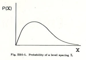
Now, if we have an average spacing, let us say D, what is the probability of a spacing, X. This question is the one which I have not solved, but perhaps I can tell you something about this which is relatively easy to see. It was pointed out at the Amsterdam conference last year that the probability is 0 at X = 0. This is rather obvious, and follows from the fact that if you have a symmetric matrix, the probability that two energy levels coincide is governed by the requirement that two parameters be 0, rather than that one parameter be 0. This was pointed out by Dr. Von Neuman and myself in an article which everybody has probably forgotten, but it is a very easy thing to show. If I take, for Instance, a two-dimensional matrix then the secular equation reads: $$E =1/2(E_1+ E_2) \pm 1/2\sqrt{(E_1 — E_2)^2 + 4V_{(12)}^2}.$$ The two roots can coincide only if the square root is equal to zero, which requires that both $E_1 - E_2 = 0$ and $V_{(12)} =0$. If you have a third order equation, which is slightly more complicated, that tells you two roots coincide, it again amounts to two equations rather than one equation. As a result, the probability is 0 and, therefore, the probability curve looks something like that in Figure 1. This is of course what is also observed. The only question is how does this look for large spacings, and the answer to this question is what I don’t know.
Dr. Hughes presented a curve which I have not seen, in which he compared an experiment with a curve which I suggested some time ago, a form $Xe^{-X^2/2}$ or something like this. Hughes found reasonably good agreement, but the agreement was good in the region of Small X, and not very good in the region of large X. Agreement in this large X region would not look so bad if the experimental curve were the theoretical curve and the theoretical curve, the experimental curve. Because if you could calculate that there should be four cases with a given spacing and you find only one, then that's unfortunate, but it is a reasonable statistical deviation. However, if you calculate that there should only be one and find four, that is a much more serious deviation and much less probable statistically.
Let me say only one more word. It is very likely that the curve in Figure 1 is a universal function. in other words, it doesn't depend on the details of the model with which you are working. There is one particular model in which the probability of the energy levels can be written down exactly. I mentioned this distribution already in Gatlinburg. It is called the Wishart distribution. Consider a set of symmetric matrixes in such a way that the diagonal element $m_{11}$ has a distribution $\exp(-m_{11}^2/4)$. In other words, the probability that this diagonal element shall assume the value $m_{11}$ is proportional to $\exp(-m_{11}^2/4)$. Then as I mentioned, and this was shown a long time ago by Wishart, the probability for the characteristic roots to be $\lambda_1, \lambda_2, \lambda_3, \ldots, \lambda_n$, if this is an $n$ dimensional matrix, is given by the expression: $$\exp(-1/2(\lambda_1^2+\lambda_2^2+..+\lambda_n^2))[(\lambda_1-\lambda_2)(\lambda_1-\lambda_3).......(\lambda_{n-1}-\lambda_n)].$$ You see again this characteristic factor which shows that the probability of two roots coinciding is 0. If you want to calculate from this formula, the probability that two successive roots have a distance X, then you have to integrate over all of them except two. This is very easy to do for the first integration, possible to do for the second integration, but when you get to the third, fourth and fifth, etc., integrations you have the same problem as in statistical mechanics, and presumably the solution of the problem will be accomplished by one of the methods of statistical mechanics. Let me only mention that I did integrate over all of them except one, and the result is $\frac{1}{2\pi}\sqrt{4n-\lambda^2}$. This is the probability that the root shall be $\lambda$. All I have to do is to integrate over one less variable than I have integrated over, but this I have not been able to do so far.
Discussion
W. HAVENS: Where does one find out about a Wishart distribution?
E. WIGNER: A Wishart distribution is given in S.S. Wilks book about statistics and I found it just by accident.

Note. Edward Teller is among other things credited as being the father of the US H-bomb. He is also one of the authors of the the famous 1953 paper entitled Equation of State Calculations by Fast Computing Machines, together with Nicholas Metropolis, Arianna Rosenbluth, Marshall Rosenbluth, and Augusta Teller, which introduced the so-called Metropolis-Hastings algorithm. Eugene Wigner received a Nobel Prize in Physics in 1963 "for his contributions to the theory of the atomic nucleus and the elementary particles, particularly through the discovery and application of fundamental symmetry principles". Wigner is often considered as a hidden genius, in comparison with Einstein.
3 Comments