This post is about the spherical ensemble of random matrices, and some of its properties in potential theory, geometry, and probability. It is at the heart of arXiv:2510.18669.
Coulomb gas. The spherical or Forrester-Krishnapur random matrix ensemble is \[ M=AB^{-1} \] where $A$ and $B$ are two independent $n\times n$ complex Ginibre matrices, namely ${(A_{jk})}_{1\leq j,k\leq n}$ and ${(B_{jk})}_{1\leq j,k\leq n}$ are iid standard complex normal random variables of law $\mathcal{N}(0,\frac{1}{2}\mathrm{Id}_2)$.
The law of $M$ is invariant by inversion : $M$ and $M^{-1}$ have the same law. The law of $M$ inherits the biunitary invariance of the complex Ginibre ensemble : invariance by multiplication from the left and from the right by deterministic unitary matrices.
The random matrix $M$ is a.s. nonnormal and its entries are dependent and heavy-tailed. When $n=1$, then $M$ is a ratio of two independent copies on the standard complex normal distribution, so its law is a complex Cauchy distribution \[ \nu=\kappa(z)\mathrm{d}z \quad\text{with density}\quad z\in\mathbb{C}\mapsto\kappa(z)=\frac{1}{\pi(1+|z|^2)^2}. \] The law $\nu$ is also known as a bivariate Student t distribution in Statistics and as a Barenblatt profile in Analysis of PDEs (fast diffusion equation). It is heavy tailed.
The spectrum of $M$ is a Coulomb gas on $\mathbb{C}$ with density $\varphi_n:\mathbb{C}^n\mapsto(0,+\infty)$ given by \[ \varphi_n(z_1,\ldots,z_n) =c_n\frac{\prod_{i < j}|z_i-z_j|^2}{\prod_{i=1}^n(1+|z_i|^2)^{n+1}} =c_n\mathrm{e}^{-(n+1)\sum_{i=1}^nQ(|z_i|)}\prod_{i < j}|z_i-z_j|^2, \] where $c_n$ is a normalizing constant, and $Q(|z|)=\log(1+|z|^2)$.
By putting this gas in a diagonal matrix and using conjugacy with an independent Haar unitary matrix, this can also be seen as the spectrum of a random normal matrix model, which should not be confused with the random non-normal matrix model $M$.
Determinantal structure. The planar Coulomb gas above is also a determinantal point process of $n$ particles on $\mathbb{C}$ endowed with the Lebesgue measure with kernel \[ (z,w)\in\mathbb{C}^2\mapsto K_n(z,w)=\sqrt{\kappa(z)\kappa(w)} n\Bigr(\frac{1+z\overline{w}}{\sqrt{(1+|z|^2)(1+|w|^2)}}\Bigr)^{n-1}. \] Contrary to certain references, we use here as a background the uniform distribution on the sphere in stereographic coordinates. This means that the joint density writes \[ \varphi_n(z_1,\ldots,z_n)=\frac{1}{n!}\det\bigr[K_n(z_i,z_j)\bigr]_{1\leq i,j\leq n}. \] The naming comes from the fact that for all $1\leq k\leq n$, the marginal density \[ (z_1,\ldots,z_k)\in\mathbb{C}^k \mapsto\varphi_{n,k}(z_1,\ldots,z_k)=\int_{\mathbb{C}^{n-k}}\varphi_n(z_1,\ldots,z_n)\mathrm{d}z_{k+1}\cdots\mathrm{d}z_n \] can be expressed using the kernel as \[ \varphi_{n,k}(z_1,\ldots,z_k) =\frac{(n-k)!}{n!}\det\bigr[K_n(z_i,z_j)\bigr]_{1\leq i,j\leq k}. \] In particular \begin{align*} \varphi_{n,n}&=\varphi_n\\ \varphi_{n,1}(w)&=\frac{1}{n}K_n(w,w)=\kappa(w)\\ \varphi_{n,2}(u,v)&=\frac{1}{n(n-1)}(K_n(u,u)K_n(v,v)-|K_n(u,v)|^2). \end{align*} This provides formulas for the mean and variance of linear statistics of the form $L_n(f)=\sum_{k=1}^nf(\lambda_k(M))$, namely \begin{align*} \mathbb{E}(L_n(f)) &=\int_{\mathbb{C}} f(w)K_n(w,w)\mathrm{d}w=n\int_{\mathbb{C}}f(w)\kappa(w)\mathrm{d}w\\ \mathrm{Var}(L_n(f)) &=\int_{\mathbb{C}}f(w)^2K_n(w,w)\mathrm{d}w -\iint_{\mathbb{C}^2}f(u)f(v)|K_n(u,v)|^2\mathrm{d}u\mathrm{d}v\\ &=n\int_{\mathbb{C}}f(w)^2\kappa(w)\mathrm{d}w -\frac{n^2}{\pi^2}\iint_{\mathbb{C}^2}f(u)f(v)\frac{|1+u\overline{v}|^{2(n-1)}}{(1+|u|^2)^{n+1}(1+|v|^2)^{n+1}}\mathrm{d}u\mathrm{d}v. \end{align*}
Spherical coordinates. Geometrically, the law $\nu$ is the image of the uniform probability measure on the sphere $\mathbb{S}^2$ by the (north pole) stereographic projection \[ T:\mathbb{S}^2\subset\mathbb{R}^3\to\mathbb{C}\cup\{\infty\}. \] More precisely, for all $x=(x_1,x_2,x_3)\in\mathbb{S}^2\setminus\{(0,0,1)\}$ and $z\in\mathbb{C}$, \[ T(x)=\frac{x_1+\mathrm{i}x_2}{1-x_3} \quad\text{and}\quad T^{-1}(z) =\frac{(2 \Re z, 2 \Im z,|z|^2-1)}{|z|^2+1}. \] In other words, this measure is the uniform probability distribution on the sphere written in stereographic coordinates. The image of the spherical ensemble by the inverse stereographic projection $T^{-1}$ is the gas on $\mathbb {S}^2$ with density with respect to the uniform measure given, up to a multiplicative normalizing constant, by \[ (x_1,\ldots,x_n)\in(\mathbb{S}^2)^n \mapsto\prod_{i < j}\|x_i-x_j\|^2_{\mathbb{R}^3}, \] hence the name of the spherical ensemble! This can be seen as a perfect two or three dimensional analogue of the circular unitary ensemble (CUE), proportional to \[ (x_1,\ldots,x_n)\in(\mathbb{S}^1)^n\subset\mathbb{C}^n\mapsto\prod_{i < j}|x_i-x_j|^2, \] that describes the spectrum of $n\times n$ Haar unitary random matrices.
Möbius transforms. This gas on $\mathbb{S}^2$ is invariant by the isometries of $\mathbb{S}^2$. When $R$ runs over the rotations of $\mathbb{S}^2$, then $T\circ R\circ T^{-1}$ runs over the maps of $\mathbb{C}\cup\{\infty\}$ of the form \[ z\mapsto\frac{\alpha z+\beta}{-\overline{\beta}z+\overline{\alpha}}, \quad (\alpha,\beta)\in\mathbb{C}^2\setminus \{(0,0)\}. \] As a consequence, if $Z$ the gas seen on $\mathbb{C}$, then for all $(\alpha,\beta) \in \mathbb C^2 \setminus \{(0,0)\}$, \[ \frac{\alpha Z+\beta}{-\overline{\beta}Z+\overline{\alpha}} \overset{\mathrm{d}}{=} Z. \] The invariance by scaling suggest to assume that $|\alpha|^2+|\beta|^2=1$, and to identify $\mathbb C \cup \{\infty\}$ with the projective line $\mathbb CP^1 = (\mathbb C^2\setminus \{(0,0)\})/\sim$ where $\sim$ is the complex colinearity equivalence relation. The geometry of this object leads to the Fubini-Study metric on $\mathbb CP^1$ induced from the Hermitian product of $\mathbb C^2$.
Quaternions, SO(3), SU(2), and PSU(2). Algebraically, the group $\mathrm{SO}(3)$ is isomorphic, by conjugacy by $T$, to the projective subgroup $\mathrm{PSU(2)}$ of $\mathrm{SU}(2)$ obtained by taking the quotient by the relation $(\alpha,\beta)\sim(-\alpha,-\beta)$, with respect to the parametrization \[ \begin{pmatrix}\alpha & \beta\\ -\overline{\beta} &\overline\alpha \end{pmatrix} \] of $\mathrm{SU}(2)$. Note that $\mathrm{SU}(2)$ is isomorphic to the unit sphere of the quaternions $\mathbb{S}^3\subset\mathbb{R}^4$ via $|\alpha|^2+|\beta|^2=1$, which leads to another way to link $\mathrm{SO}(3)$ with $\mathrm{SU}(2)$. \[ z\mapsto\frac{\alpha z+\beta}{-\overline{\beta}z+\overline{\alpha}}, \quad \alpha,\beta\in\mathbb{C},\quad |\alpha|^2+|\beta|^2=1. \] In particular, for all $z_0\in\mathbb{C}$, a Möbius transform that maps $z_0$ to $0$ is \[ z\mapsto M_{z_0}(z)=\frac{z-z_0}{\overline{z_0}z+1}. \] As a consequence, if $Z$ is the gas seen on $\mathbb{C}$, then for all $z_0\in\mathbb{C}$, \[ M_{z_0}(Z)=\frac{Z-z_0}{\overline{z_0}Z+1} \overset{\mathrm{d}}{=} Z. \] Since $M_{z_0}(z_0)=0$ and $M'_{z_0}(z_0)=\frac{1}{1+|z_0|^2}$, a version of the delta method for random point processes gives that the local behavior of $\frac{Z-z_0}{1+|z_0|^2}$ near $z_0$ is equal to the one of $Z$ near $0$.
Kostlan observation and spectral radius. If $Z_n=(Z_{n,1},\ldots,Z_{n,n})$ is the gas seen as a random vector of $\mathbb{C}^n$, then the determinantal structure and rotational invariance give \[ \{|Z_{n,1}|,\ldots,|Z_{n,n}|\}\overset{\mathrm{d}}{=}\{\xi_{n,1},\ldots,\xi_{n,n}\} \] where $\xi_{n,1},\ldots,\xi_{n,n}$ are independent and $\xi_{n,k}$ has density proportional to \[ x\geq0\mapsto x^{2k-1}\mathrm{e}^{-(n+1)Q(x)}=\frac{x^{2k-1}}{(1+x^2)^{n+1}}. \] The random variable $\xi_{n,k}^2$ has density proportional to \[ x\geq0\mapsto\frac{x^{k-1}}{(1+x)^{n+1}}. \] We recognize a Beta prime (or inverse Beta or Beta of the second kind) law of density \[ x\geq0\mapsto\frac{\Gamma(a+b)}{\Gamma(a)\Gamma(b)}\frac{x^{a-1}}{(1+x)^{a+b}}, \] with $a=k$ and $b=n-k+1$, which is also the law of $B/(1-B)$ when $B\sim\mathrm{Beta}(a,b)$, and also the law of $G_a/G_b$ were $G_a\sim\mathrm{Gamma}(a,\lambda)$ and $G_b\sim\mathrm{Gamma}(b,\lambda)$ are independent and $\lambda > 0$ is an arbitrary scale parameter.
For any fixed $k$, since $\mathrm{Gamma}(n-k+1,1)=\mathrm{Exp}(1)^{*(n-k+1)}$, the law of large numbers gives $n/S_{n,k}\to1$ a.s. as $n\to\infty$, where $S_{n,k}\sim\mathrm{Gamma}(n-k+1)$. It follows that \[ \frac{n}{\xi_{n,n-k}^2} \xrightarrow[n\to\infty]{\mathrm{d}} \mathrm{Gamma}(k,1), \] and more generally, the fluctuations of the spectral radius are given by \[ \frac{1}{\sqrt{n}}\rho(M) =\frac{1}{\sqrt{n}}\max_{1\leq k\leq n}|Z_{n,k}| \overset{\mathrm{d}}{=} \frac{1}{\sqrt{n}}\max_{1\leq k\leq n}\xi_{n,k} \xrightarrow[n\to\infty]{\mathrm{d}} \mathrm{Law}\Bigr(\max_{k\geq1}\frac{1}{\sqrt{\gamma_k}}\Bigr) \] where ${(\gamma_k)}_{k\geq1}$ are independent with $\gamma_k\sim\mathrm{Gamma}(k,1)$.
Equilibrium measure. Regarding high dimensional asymptotic analysis, a.s. \[ \mu_{M} \overset{\mathrm{d}}{=}\frac{1}{n}\sum_{k=1}^n\delta_{Z_{n,k}} \xrightarrow[n\to\infty]{\text{weak}} \frac{\Delta Q(\left|\cdot\right|)}{2\pi}\mathrm{d}z =\frac{\mathrm{d}z}{\pi(1+|z|^2)^2} =\mathrm{\nu}, \] The average version is easy to check using logarithmic potential and remains valid non asymptotically. Indeed, for all $z\in\mathbb{C}$, $B$ and $A-zB$ are correlated, but by Gaussianity, \[ (M-z\mathrm{Id})B =A-zB \overset{\mathrm{d}}{=} \sqrt{1+|z|^2}A. \] Therefore, for all $z\in\mathbb{C}$, in $[-\infty,+\infty)$, \[ \mathbb{E}\log|\det(M-z\mathrm{Id})|+\mathbb{E}\log|\det(B)| =n\log\sqrt{1+|z|^2}+\mathbb{E}\log|\det(A)|. \] Finally, by applying the operator $\frac{1}{2\pi}\Delta$ in the sense of distributions, we obtain the stunning non-asymptotic formula \[ \mathbb{E}\mu_M=\frac{\Delta\log(1+|z|^2)}{4\pi}\mathrm{d}z=\frac{\mathrm{d}z}{\pi(1+|z|^2)^2}=\mathrm{\nu}. \] Alternatively, this formula can be extracted from the determinantal structure, namely \[ \mathbb{E}\mu_M=\frac{1}{n}K_n(z,z)\mathrm{d}z=\kappa(z)\mathrm{d}z=\nu. \] Alternatively, we could simply use the fact that the uniform distribution on $\mathbb{S}^2$ is the unique distribution on $\mathbb{S}^2$ invariant by all rotations, together with the fact that its image by the stereographic projection $T$ is precisely $\nu$ !
More generally, if $A$ and $B$ are Girko matrices, then $A-zB=\sqrt{1+|z|^2}C_z$ where $C_z$ is a Girko matrix, but with a law that depends on $z$ in general, except in the Gaussian case. Also the argument above works only in the Ginibre case.
Coulomb kernel. Let is consider $g:\mathbb{C}\times\mathbb{C}\mapsto(-\infty,+\infty]$ defined for $z,w\in\mathbb{C}$ by \[ g(z,w)=\log|z-w|-\tfrac{1}{2}\log(1+|z|^2)-\tfrac{1}{2}\log(1+|w|^2). \] It is the Coulomb kernel of the two-sphere $\mathbb{S}^2$ in stereographic coordinates since \[ \Delta g(\cdot,w)\overset{\mathcal{D}'}{=}2\pi(\delta_w-\nu). \] Since $2\langle z,w\rangle_{\mathbb{R}^2}=\bar{z}w+z\bar{w}$ for all $z,w\in\mathbb{C}^2\equiv\mathbb{R}^2$, we get, when $T(x)=z$ and $T(y)=w$, \begin{align*} 1-\langle x,y\rangle_{\mathbb{R}^3} &=1-\langle T^{-1}(z),T^{-1}(w)\rangle_{\mathbb{R}^3}\\ &=1-\frac{2(\bar{z}w+z\bar{w})+(|z|^2-1)(|w|^2-1)}{(1+|z|^2)(1+|w|^2)}\\ &=\frac{2|z-w|^2}{(1+|z|^2)(1+|w|^2)}. \end{align*} Also, a natural alternative definition of the Coulomb kernel of $\mathbb{S}^2$ is, for $x,y\in\mathbb{S}^2\subset\mathbb{R}^3$, \begin{align*} \mathfrak{G}(x,y) &= 2\log\|x-y\|_{\mathbb{R}^3}\\ &=\log\bigr(1-\langle x,y\rangle_{\mathbb{R}^3}\bigr)+\log(2)\\ &=2g(z,w)+2\log(2). \end{align*} It is symmetric $\mathfrak{G}(x,y)=\mathfrak{G}(y,x)$, exhibits logarithmic divergence on the diagonal, and \[ \Delta_{\mathbb{S}^2} \mathfrak{G}(\cdot,y) \overset{\mathcal{D}'}{=} 4\pi\Bigr(\delta_y -\frac{\mathrm{d}x}{4\pi}\Bigr) \] for $y\in\mathbb{S}^2$, where $\Delta_{\mathbb{S}^2}$ is the Laplace-Beltrami operator on $\mathbb{S}^2$. Moreover, we have \[ \int g(z,w)\mathrm{d}\nu(w) =-\int\frac{1}{2}\log(1+|w|^2)\mathrm{d}\nu(w) =-\frac{1}{2}, \] for $z\in\mathbb{C}$ which gives, in particular, for $x\in\mathbb{S}^2$, \[ \int\mathfrak{G}(x,y)\mathrm{d}y =2\log(2)-1. \]
Central Limit Theorem. Since \[ \log|\det(M)|=\log|\det(A)|-\log|\det(B)| \] and since $A$ and $B$ are independent and can be Hermitized into complex square Wishart matrices or factorized using the Choleski-Bartlett decomposition, a CLT for $\log|\det(M)|$ boils down to a CLT for independent $\chi^2$ variables. It can also be obtained using the Kostlan observation. More precisely, we get \[ \frac{\log|\det(M)|}{\sqrt{\frac{1}{2}\log(n)}} \xrightarrow[n\to\infty]{\mathrm{d}} \mathcal{N}(0,1). \] We have $\mathbb{E}\log|\det(M)|=0$ since the law of $M$ is invariant by inversion.
Further reading.
- D. Chafaï and S. Péché
A note on the second order universality at the edge of Coulomb gases on the plane
J. Stat. Phys., 156(2) (2014) - P. J. Forrester
Log-gases and random matrices
Princeton University Press (2010) - P. J. Forrester and A. Mays
Pfaffian point process for the Gaussian real generalised eigenvalue problem
Probab. Theory Relat. Fields 154(1-2) (2012) - I. M. Gel’fand, R. A. Minlos, and Z. Y. Shapiro
Representations of the rotation and Lorentz groups and their applications
Translated from the Russian by G. Cummins and T. Boddington
Oxford University Press (1963) - A. Hardy
A note on large deviations for 2D Coulomb gas with weakly confining potential
Electron. Commun. Probab. 17:19 (2012) - J. B. Hough, M. Krishnapur, Y. Peres, and B. Virág
Zeros of Gaussian analytic functions and determinantal point processes
American Mathematical Society (2009) - D. Huybrechts
Complex geometry. An introduction
Universitext Springer (2005) - E. Kostlan
On the spectra of Gaussian matrices
Linear Algebra Appl. 162/164 (1992) - M. Krishnapur
From random matrices to random analytic functions
Ann. Probab. 37(1) (2009) - T. Needham
Visual complex analysis. 25th anniversary edition, with a new foreword by Roger Penrose
Oxford: Oxford University (2023) - B. Rider
A limit theorem at the edge of a non-Hermitian random matrix ensemble
J. Phys. A, Math. Gen. 36(12) (2003)
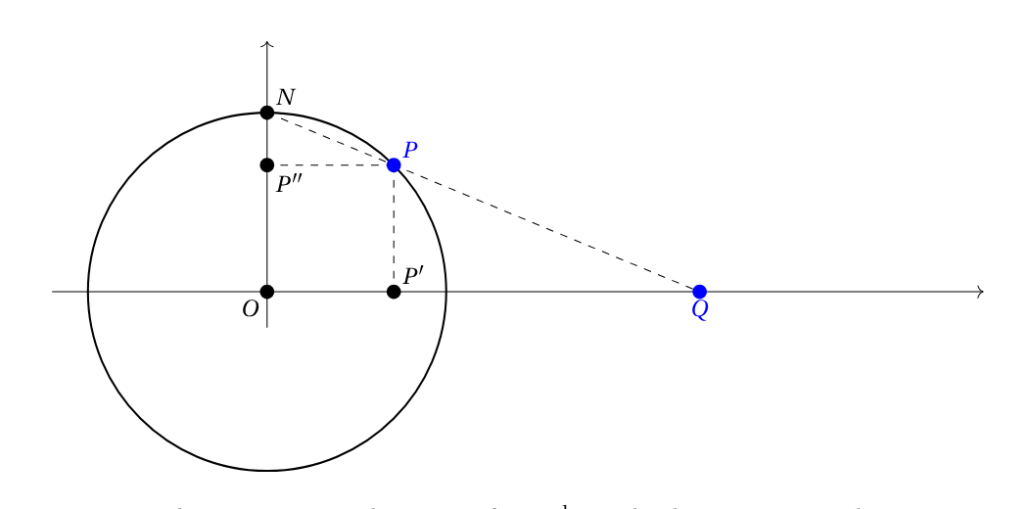
Appendix. The point $Q\in\mathbb{R}$ is the image of $P\in\mathbb{S}^1\setminus\{N\}$ by the 1D stereographic projection $T$ with respect of the north pole $N$. The image of $N$ is $\infty$.
- The Pythagoras Theorem for the triangle $ONQ$ gives $1+OQ^2=NQ^2$ since $ON=1$.
- The Thales Theorem for the couple of alignments $QP'O$ and $QPN$ gives \[ \frac{OQ}{OP'}=\frac{NQ}{NP}. \] Combining with the previous result and eliminating $NQ$ gives \[ 1+OQ^2=\frac{OQ^2 NP^2}{OP'^2} \quad\text{hence}\quad OQ^2=\frac{OP'^2}{OP'^2-NP^2}. \]
- The Pythagoras Theorem again, this time for the triangle $NPP''$, gives \[ NP^2=PP''^2+NP''^2=OP'^2+NP''^2, \quad\text{hence}\quad OQ^2=\frac{OP'^2}{NP''^2}, \] which is the 1D formula $T(x)=x_1/(1-x_2)$ for $(x_1,x_2)\in\mathbb{S}^1\setminus\{e_2\}$, with the Cartesian transcription $O=0$, $N=e_2$, $P=x$, $Q=T(x)$.
The 2D formula $T(x)=(x_1,x_2)/(1-x_3)$ for $(x_1,x_2,x_3)\in\mathbb{S}^2\setminus\{e_3\}$ follows from the 1D formula by the coplanarity of $0$, $e_3$, $x$, and $T(x)$. More generally, in arbitrary dimension $d\geq1$, $T(x)=(x_1,\ldots,x_{d-1})/(1-x_d)$, $x\in\mathbb{S}^{d-1}\setminus\{e_d\}$.