Aspects of the Complex Ginibre Ensemble

This post is devoted to the Complex Ginibre Ensemble, the subject of an expository talk that I gave few months ago. Let ${(G_{i,j})_{i,j\geq1}}$ be an infinite table of i.i.d. random variables on ${\mathbb{C}\equiv\mathbb{R}^2}$ with ${G_{11}\sim\mathcal{N}(0,\frac{1}{2}I_2)}$. The Lebesgue density of the ${n\times n}$ random matrix ${\mathbf{G}=(G_{i,j})_{1\leq i,j\leq n}}$ in ${\mathcal{M}_n(\mathbb{C})\equiv\mathbb{C}^{n\times n}}$ is

$$\mathbf{A}\in\mathcal{M}_n(\mathbb{C}) \mapsto \pi^{-n^2}e^{-\sum_{i,j=1}^n|\mathbf{A}_{ij}|^2} = \pi^{-n^2}e^{-\mathrm{Tr}(\mathbf{A}\mathbf{A}^*)} \ \ \ \ \ (1)$$

where ${\mathbf{A}^*}$ the conjugate-transpose of ${\mathbf{A}}$. We say that ${\mathbf{G}}$ belong to the Complex Ginibre Ensemble. This law is unitary invariant, in the sense that if ${\mathbf{U}}$ and ${\mathbf{V}}$ are ${n\times n}$ unitary matrices then ${\mathbf{U}\mathbf{G}\mathbf{V}}$ and ${\mathbf{G}}$ are equally distributed. The entry-wise and matrix-wise real and imaginary parts of ${\mathbf{G}}$ are independent and belong to the Gaussian Unitary Ensemble (GUE) of Gaussian random Hermitian matrices (the converse is also true).

The eigenvalues ${\lambda_1(\mathbf{A}),\ldots,\lambda_n(\mathbf{A})}$ of a matrix ${\mathbf{A}\in\mathcal{M}_n(\mathbb{C})}$ are the roots in ${\mathbb{C}}$ of its characteristic polynomial ${P_\mathbf{A}(z)=\det(\mathbf{A}-z\mathbf{I})}$, labeled so that ${|\lambda_1(\mathbf{A})|\geq\cdots\geq|\lambda_n(\mathbf{A})|}$ with growing phases.

Lemma 1 (Diagonalizability) For every ${n\geq1}$, the set of elements of ${\mathcal{M}_n(\mathbb{C})}$ with multiple eigenvalues has zero Lebesgue measure in ${\mathbb{C}^{n\times n}}$. In particular, the set of nondiagonalizable elements of ${\mathcal{M}_n(\mathbb{C})}$ has zero Lebesgue measure in ${\mathbb{C}^{n\times n}}$.

Proof: If ${\mathbf{A}\in\mathcal{M}_n(\mathbb{C})}$ has characteristic polynomial

$$P_\mathbf{A}(z)=z^n+a_{n-1}z^{n-1}+\cdots+a_0,$$

then ${a_0,\ldots,a_{n-1}}$ are polynomials functions of ${\mathbf{A}}$. The resultant ${R(P_\mathbf{A},P'_\mathbf{A})}$ of ${P_\mathbf{A},P'_\mathbf{A}}$, called the discriminant of ${P_\mathbf{A}}$, is the determinant of the ${(2n-1)\times(2n-1)}$ Sylvester matrix of ${P_\mathbf{A},P'_\mathbf{A}}$. It is a polynomial in ${a_0,\ldots,a_{n-1}}$. We have also the Vandermonde formula

$$|R(P_\mathbf{A},P'_\mathbf{A})|=\prod_{i{<}j}|\lambda_i(\mathbf{A})-\lambda_j(\mathbf{A})|^2.$$

Consequently, ${\mathbf{A}}$ has all eigenvalues distinct if and only if ${\mathbf{A}}$ lies outside the polynomial hyper-surface ${\{\mathbf{A}\in\mathbb{C}^{n\times n}:R(P_\mathbf{A},P'_\mathbf{A})=0\}}$. ☐

Since the law of ${\mathbf{G}}$ is absolutely continuous, from lemma 1, we get that a.s. ${\mathbf{G}\mathbf{G}^*\neq \mathbf{G}^*\mathbf{G}}$ (nonnormality) but ${\mathbf{G}}$ is diagonalizable with distinct eigenvalues. Note that if ${\mathbf{G}=\mathbf{U}\mathbf{T}\mathbf{U}^*}$ is the Schur unitary decomposition where ${\mathbf{U}}$ is unitary and ${\mathbf{T}}$ is upper triangular, then ${\mathbf{T}=\mathbf{D}+\mathbf{N}}$ with ${\mathbf{D}=\mathrm{diag}(\lambda_1(\mathbf{G}),\ldots,\lambda_n(\mathbf{G}))}$ and

$$\mathrm{Tr}(\mathbf{G}\mathbf{G}^*) =\mathrm{Tr}(\mathbf{D}\mathbf{D}^*) +\mathrm{Tr}(\mathbf{N}\mathbf{N}^*).$$

Following Ginibre, one may compute the joint density of the eigenvalues by integrating (1) over the non spectral variables ${\mathbf{U}}$ and ${\mathbf{N}}$. The result is stated in Theorem 2 below. The law of ${\mathbf{G}}$ is invariant by the multiplication of the entries with a common phase, and thus the law spectrum of ${\mathbf{G}}$ is rotationally invariant in ${\mathbb{C}^n}$. In the sequel we set

$$\Delta_n:=\{(z_1,\ldots,z_n)\in\mathbb{C}^n:|z_1|\geq\cdots\geq|z_n|\}.$$

Theorem 2 (Spectrum law) ${(\lambda_1(\mathbf{G}),\ldots,\lambda_n(\mathbf{G}))}$ has density ${n!\varphi_n\mathbf{1}_{\Delta_n}}$ where

$$\varphi_n(z_1,\ldots,z_n)=\frac{\pi^{-n}}{\prod_{k=1}^nk!} \exp\left(-\sum_{k=1}^n|z_k|^2\right)\prod_{1\leq i{<}j\leq n}|z_i-z_j|^2.$$

In particular, for every symmetric Borel function ${F:\mathbb{C}^n\rightarrow\mathbb{R}}$,

$$\mathbb{E}[F(\lambda_1(\mathbf{G}),\ldots,\lambda_n(\mathbf{G}))] =\int_{\mathbb{C}^n}\!F(z_1,\ldots,z_n)\varphi_n(z_1,\ldots,z_n)\,dz_1\cdots dz_n.$$

We will use Theorem 2 with symmetric functions of the form

$$F(z_1,\ldots,z_n) =\sum_{i_1,\ldots,i_k \text{ distinct}}f(z_{i_1})\cdots f(z_{i_k}).$$

The Vandermonde determinant comes from the Jacobian of the diagonalization, and can be interpreted as an electrostatic repulsion. The spectrum is a Gaussian determinantal process. One may also take a look at the fourth chapter of the book by Hough, Krishnapur, Peres, and Virag for a generalization to zeros of Gaussian analytic functions. Theorem 2 is reported in chapter 15 of Mehta's book. Ginibre considered additionally the case where ${\mathbb{C}}$ is replaced by ${\mathbb{R}}$ or by the quaternions. These two cases are less studied than the complex case, due to their peculiarities. For instance, for the real Gaussian case, and following Edelman (Corollary 7.2), the probability that the ${n\times n}$ matrix has all its eigenvalues real is ${2^{-n(n-1)/4}}$, see also Akemann and Kanzieper. The whole spectrum does not have a density in ${\mathbb{C}^n}$ in this case!

Theorem 3 (${k}$-points correlations) Let ${z\in\mathbb{C}\mapsto\gamma(z)=\pi^{-1}e^{-|z|^2}}$ be the density of the standard Gaussian law ${\mathcal{N}(0,\frac{1}{2}I_2)}$ on ${\mathbb{C}}$. Then for every ${1\leq k\leq n}$, the ${k}$-point correlation''

$$\varphi_{n,k}(z_1,\ldots,z_k) := \int_{\mathbb{C}^{n-k}}\!\varphi_n(z_1,\ldots,z_k)\,dz_{k+1}\cdots dz_n$$

satisfies to

$$\varphi_{n,k}(z_1,\ldots,z_k) = \frac{(n-k)!}{n!}\gamma(z_1)\cdots\gamma(z_k) \det\left[K(z_i,z_j)\right]_{1\leq i,j\leq k}$$

where

$$K(z_i,z_j) :=\sum_{\ell=0}^{n-1}\frac{(z_iz_j^*)^\ell}{\ell!} =\sum_{\ell=0}^{n-1}H_\ell(z_i)H_\ell(z_j)^* \quad\text{with}\quad H_\ell(z):=\frac{1}{\sqrt{\ell!}}z^\ell.$$

In particular, by taking ${k=n}$ we get

$$\varphi_{n,n}(z_1,\ldots,z_n) =\varphi_n(z_1,\ldots,z_n) =\frac{1}{n!}\gamma(z_1)\cdots\gamma(z_n)\det\left[K(z_i,z_j)\right]_{1\leq i,j\leq n}.$$

Proof: Calculations made by Mehta (chapter 15 page 271 equation 15.1.29) using

$$\prod_{1\leq i{<}j\leq n}|z_i-z_j|^2 =\prod_{1\leq i{<}j\leq n}(z_i-z_j)\prod_{1\leq i{<}j\leq n}(z_i-z_j)^*$$

and

$$\det\left[z_j^{i-1}\right]_{1\leq i,j\leq k}\det\left[(z_j^*)^{i-1}\right]_{1\leq i,j\leq k} =\frac{\prod_{j=1}^kj!}{n!}\det\left[K(z_i,z_j)\right]_{1\leq i,j\leq k}.$$

☐

Recall that the empirical spectral distribution of an ${n\times n}$ matrix ${A}$ is given by

$$\mu_\mathbf{A}:=\frac{1}{n}\sum_{k=1}^n\delta_{\lambda_k(\mathbf{A})}.$$

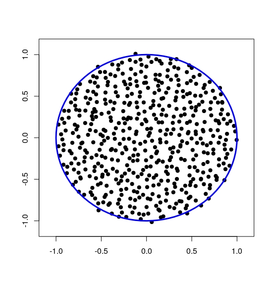
Theorem 4 (Mean Circular Law) For every continuous bounded function ${f:\mathbb{C}\rightarrow\mathbb{R}}$,

$$\lim_{n\rightarrow\infty}\mathbb{E}\left[\int\!f\,d\mu_{\frac{1}{\sqrt{n}}\mathbf{G}}\right] =\pi^{-1}\int_{|z|\leq 1}\!f(z)\,dxdy.$$

Proof: From Theorem 3, with ${k=1}$, we get that the density of ${\mathbb{E}\mu_{\mathbf{G}}}$ is

$$\varphi_{n,1}: z\mapsto \gamma(z)\left(\frac{1}{n}\sum_{\ell=0}^{n-1}|H_\ell|^2(z)\right) =\frac{1}{n\pi}e^{-|z|^2}\sum_{\ell=0}^{n-1}\frac{|z|^{2\ell}}{\ell!}.$$

Following Mehta (chapter 15 page 272), by elementary calculus, for every compact ${C\subset\mathbb{C}}$,

$$\lim_{n\rightarrow\infty}\sup_{z\in C} \left|n\varphi_{n,1}(\sqrt{n}z)-\pi^{-1}\mathbf{1}_{[0,1]}(|z|)\right|=0.$$

The ${n}$ in front of ${\varphi_{n,1}}$ is due to the fact that we are on the complex plane ${\mathbb{C}=\mathbb{R}^2}$ and thus ${d\sqrt{n}xd\sqrt{n}y=ndxdy}$. Here is the start of the elementary calculus: for ${r^2<n}$,

$$e^{r^2}-\sum_{\ell=0}^{n-1}\frac{r^{2\ell}}{\ell!} =\sum_{\ell=n}^\infty\frac{r^{2\ell}}{\ell!} \leq \frac{r^{2n}}{n!}\sum_{\ell=0}^\infty\frac{r^{2\ell}}{(n+1)^\ell} =\frac{r^{2n}}{n!}\frac{n+1}{n+1-r^2}$$

while for ${r^2>n}$,

$$\sum_{\ell=0}^{n-1}\frac{r^{2\ell}}{\ell!} \leq\frac{r^{2(n-1)}}{(n-1)!}\sum_{\ell=0}^{n-1}\left(\frac{n-1}{r^2}\right)^\ell \leq \frac{r^{2(n-1)}}{(n-1)!}\frac{r^2}{r^2-n+1}.$$

This leads to the result by taking ${r^2:=|\sqrt{n}z|^2}$. ☐

The real Gaussian version of Theorem 4 was established by Edelman (theorem 6.3). The sequence ${(H_k)_{k\in\mathbb{N}}}$ forms an orthonormal basis of square integrable analytic functions on ${\mathbb{C}}$ for the standard Gaussian on ${\mathbb{C}}$. The uniform law on the unit disc (known as the circular law) is the law of ${\sqrt{V}e^{2i\pi W}}$ where ${V}$ and ${W}$ are i.i.d. uniform random variables on the ${[0,1]}$. Ledoux makes use of this point of view for his interpolation between complex Ginibre and GUE via the Girko elliptic laws (see also Johansson).

Theorem 5 (Strong Circular Law) Almost surely, for all continuous bounded ${f:\mathbb{C}\rightarrow\mathbb{R}}$,

$$\lim_{n\rightarrow\infty}\int\!f\,d\mu_{\frac{1}{\sqrt{n}}\mathbf{G}} = \pi^{-1}\int_{|z|\leq 1}\!f(z)\,dxdy.$$

Proof: We reproduce Silverstein's argument, published by Hwang. The argument is similar to the proof of the strong law of large numbers for i.i.d. random variables with finite fourth moment. It suffices to establish the result for compactly supported continuous bounded functions. Let us pick such a function ${f}$ and set

$$S_n:=\int_{\mathbb{C}}\!f\,d\mu_{\frac{1}{\sqrt{n}}\mathbf{G}} \quad\text{and}\quad S_\infty:=\pi^{-1}\int_{|z|\leq 1}\!f(z)\,dxdy.$$

Suppose for now that we have

$$\mathbb{E}[\left(S_n-\mathbb{E} S_n\right)^4]=O(n^{-2}). \ \ \ \ \ (2)$$

By monotone convergence,

$$\mathbb{E}\sum_{n=1}^\infty\left(S_n-\mathbb{E} S_n\right)^4 =\sum_{n=1}^\infty\mathbb{E}[\left(S_n-\mathbb{E} S_n\right)^4]<\infty$$

and consequently ${\sum_{n=1}^\infty\left(S_n-\mathbb{E} S_n\right)^4<\infty}$ a.s. which implies ${\lim_{n\rightarrow\infty}S_n-\mathbb{E} S_n=0}$ a.s. Since ${\lim_{n\rightarrow\infty}\mathbb{E} S_n=S_\infty}$ by theorem 4, we get ${\lim_{n\rightarrow\infty}S_n=S_\infty}$ a.s. Finally, one can swap the universal quantifiers on ${\omega}$ and ${f}$ thanks to the separability of ${\mathcal{C}_c(\mathbb{C},\mathbb{R})}$. To establish (2), we set

$$S_n-\mathbb{E} S_n=\frac{1}{n}\sum_{i=1}^nZ_i \quad\text{with}\quad Z_i:=f\left(\lambda_i\left(\frac{1}{\sqrt{n}}\mathbf{G}\right)\right).$$

Next, we obtain, with ${\sum_{i_1,\ldots}}$ running over distinct indices in ${1,\ldots,n}$,

$$\mathbb{E}\left[\left(S_n-\mathbb{E} S_n\right)^4\right] =\frac{1}{n^4}\sum_{i_1}\mathbb{E}[Z_{i_1}^4]$$

$$+\frac{4}{n^4}\sum_{i_1,i_2}\mathbb{E}[Z_{i_1}Z_{i_2}^3]$$

$$+\frac{3}{n^4}\sum_{i_1,i_2}\mathbb{E}[Z_{i_1}^2Z_{i_2}^2]$$

$$+\frac{6}{n^4}\sum_{i_1,i_2,i_3}\mathbb{E}[Z_{i_1}Z_{i_2}Z_{i_3}^2]$$

$$+\frac{1}{n^4}\sum_{i_1,i_2,i_3,i_3,i_4}\!\!\!\!\!\!\mathbb{E}[Z_{i_1}Z_{i_3}Z_{i_3}Z_{i_4}].$$

The first three terms of the right hand side are ${O(n^{-2})}$ since ${\max_{1\leq i\leq n}|Z_i|\leq\Vert f\Vert_\infty}$. Finally, some calculus using the expressions of ${\varphi_{n,3}}$ and ${\varphi_{n,4}}$ provided by Theorem 3 allows to show that the remaining two terms are also ${O(n^{-2})}$. See Hwang (page 151). ☐

Following Kostlan, the integration of the phases in the joint density of the spectrum given by Theorem 2 leads to theorem 6 below. See also Rider and the book by Hough, Krishnapur, Peres, and Virag for a generalization to determinental processes.

Theorem 6 (Layers) If ${Z_{1},\ldots,Z_{n}}$ are independent with ${Z_k^2\sim\Gamma(k,1)}$ for every ${k}$, then

$$\left\{|\lambda_1(\mathbf{G})|,\ldots,|\lambda_n(\mathbf{G})|\right\} \overset{d}{=} \left\{Z_{1},\ldots,Z_{n}\right\}.$$

Note that ${(\sqrt{2}Z_k)^2\sim\chi^2(2k)}$ which is useful for ${\sqrt{2}\mathbf{G}}$. Since ${Z_k^2\overset{d}{=}E_1+\cdots+E_k}$ where ${E_1,\ldots,E_k}$ are i.i.d. exponential random variables of unit mean, we get, for every ${r>0}$,

$$\mathbb{P}\left(\rho(\mathbf{G})\leq \sqrt{n}r\right) =\prod_{1\leq k\leq n}\mathbb{P}\left(\frac{E_1+\cdots+E_k}{n}\leq r^2\right)$$

where ${\rho(\mathbf{G})=\max_{1\leq i\leq n}|\lambda_i(\mathbf{G})|=|\lambda_1(\mathbf{G})|}$ is the spectral radius of ${\mathbf{G}}$.

The law of large numbers suggests that ${r=1}$ is a critical value. The central limit theorem suggests that ${n^{-1/2}\rho(\mathbf{G})}$ behaves when ${n\gg1}$ as the maximum of a standard Gaussian i.i.d sample, for which the fluctuations follow the Gumbel law. A quantitative central limit theorem and the Borel-Cantelli lemma provides the follow result. The full proof is in Rider.

Theorem 7 (Convergence and fluctuation of the spectral radius)

$$\mathbb{P}\left(\lim_{n\rightarrow\infty}\frac{1}{\sqrt{n}}\rho(\mathbf{G})=1\right)=1.$$

Moreover, if ${\gamma_n:=\log(n/2\pi)-2\log(\log(n))}$ then

$$\sqrt{4n\gamma_n} \left(\frac{1}{\sqrt{n}}\rho(\mathbf{G})-1-\sqrt{\frac{\gamma_n}{4n}}\right) \overset{d}{\underset{n\rightarrow\infty}{\longrightarrow}} \mathcal{G}.$$

where ${\mathcal{G}}$ is the Gumbel law with cumulative distribution function ${x\mapsto e^{-e^{-x}}}$ on ${\mathbb{R}}$.

The convergence of the spectral radius was obtained by Mehta (chapter 15 page 271 equation 15.1.27) by integrating the joint density of the spectrum of Theorem 2 over the set ${\bigcap_{1\leq i\leq n}\{|\lambda_i|>r\}}$. The same argument is reproduced by Hwang (pages 149-150). Let us give now an alternative derivation of Theorem 4. From Theorem 7, the sequence ${(\mathbb{E}\mu_{n^{-1/2}\mathbf{G}})_{n\geq1}}$ is tight and every adherence value ${\mu}$ is supported in the unit disc. From Theorem 2, such a ${\mu}$ is rotationally invariant, and from Theorem 6, the image of ${\mu}$ by ${z\in\mathbb{C}\mapsto|z|}$ has density ${r\mapsto 2r\mathbf{1}_{[0,1]}(r)}$ (use moments!). Theorem 4 follows immediately.

Note that the recent book of Forrester contains many computations for the Ginibre Ensemble. See also the chapter by Khoruzhenko and Sommers in the Oxford Handbook of Random Matrices.