This post is devoted to a formula for the Wasserstein $\mathrm{W}_2$ distance between two elements of the position-scale family of an elliptic distribution. This includes for instance Barenblatt profiles, and in particular multivariate Student t distributions (heavy tailed), and multivariate Gaussians.
Let us recall that the Wasserstein or Kantorovich or Monge $\mathrm{W}_2$ distance between two probability measures $\mu$ and $\nu$ on $\mathbb{R}^d$ with finite second moment is \[ \mathrm{W}_2(\mu,\nu)=\sqrt{\iint_{\pi}|x-y|^2\mathrm{d}\pi(x,y)} \] where the infimum runs over all probability measures $\pi$ on the product space $\mathbb{R}^d\times\mathbb{R}^d$ with marginal distributions $\mu$ and $\nu$, and where $\left|\cdot\right|$ denotes the Euclidean norm.
Wasserstein for position-scale transformation. Let $\mu$ be a probability measure on $\mathbb{R}^d$ with finite second moment, and $\nu$ the image or pushforward of $\mu$ by an affine map \[ x\mapsto T(x)=Ax+h \] where $h$ is a vector of $\mathbb{R}^d$ and $A$ is a positive-semidefinite $d\times d$ symmetric matrix. Then \[ \mathrm{W}_2^2(\mu,\nu) =\mathrm{Trace}((A-I)^2M_\mu) +2\langle(A-I)m_\mu,h\rangle+|h|^2 \] where \[ m_\mu:=\int x\mathrm{d}\mu(x) \quad\text{and}\quad M_\mu:=\int xx^\top\mathrm{d}\mu(x) \] are the first two moments of $\mu$. Alternatively, \[ \mathrm{W}_2^2(\mu,\nu)=\mathrm{Tr}(\Sigma_\mu+\Sigma_\nu-2A\Sigma_\mu)+|m_\mu-m_\nu|^2, \] where $\Sigma_\mu$ and $\Sigma_\nu$ are the covariance matrices of $\mu$ and $\nu$, and $m_\nu$ is the mean of $\nu$.
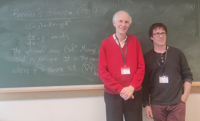
Proof. First of all, an affine map is the gradient of a convex function if and only if the matrix of the linear part is symmetric positive semidefinite. Second, the uniqueness in the Brenier theorem on optimal transportation states that if a transportation map is the gradient of a convex function, then it is the optimal transportation map. It remains to use the fact that \[ \mathrm{W}_2^2(\mu,\nu) =\int|T(x)-x|^2\mathrm{d}\mu(x) =\int(|(A-I)x|^2+2\langle(A-I)x,h\rangle+|h|^2)\mathrm{d}\mu(x). \] This gives the first formula for $\mathrm{W}_2$. The second comes from $m_\nu=Am_\mu+h$, $\Sigma_\mu=M_\mu+m_\mu m_\mu^\top$, and $\Sigma_\nu=A\Sigma_\mu A$. We note also that $T(x)=A(x-m_\mu)+m_\nu$.
About location-scale families of elliptic distributions. It turns out that the location-scale family of a rotationally invariant probability distribution is parametrized by the mean and covariance. We speak about elliptic families or elliptic distributions. Basic examples are given by Gaussian distributions and more generally Barenblatt profiles : on $\mathbb{R}^d$, $d\geq1$, for $r > 0$, $p\in(-\infty,0)\cup(\frac{d}{2},+\infty)$, and a normalizing constant $c > 0$, \[ x\in\mathbb{R}^n \mapsto\frac{c}{\Bigr(r^2+\frac{|x|^2}{p}\Bigr)_+^p}. \] For $p > \frac{d}{2}$, it is a multivariate Student t distribution. When $p\to+\infty$, it boils down to an isotropic multivariate Gaussian. For $p < 0$, it has compact support and appears as a sort of multivariate Beta distribution, related to spherical projections. The two regimes are unified at $m=1$ instead of $p=\infty$ by the Barenblatt parametrization $p=\frac{1}{1-m}$, $m > 1-\frac{2}{d}$. This is related to the nonlinear partial differential equation $\partial_tu=\Delta(u^m)$, known as the fast diffusion equation for $m<1$, the heat equation for $m=1$, and the porous medium equation for $m>1$.
For elliptic families, the affine map can be expressed in terms of the covariance matrices, as expressed below. The formula for the distance based on means and covariances, well known for Gaussians, works actually for elliptic families !
Wasserstein distance for elliptic families. Let $\eta$ be a rotationally invariant probability measure on $\mathbb{R}^d$, with zero mean and identity covariance matrix. Let $\mu$ and $\nu$ be two probability measures in the location-scale family of $\eta$, namely images or pushforwards of $\eta$ by the affine maps \begin{equation} x\mapsto T_\mu(x):=m_\mu+\sqrt{\Sigma_\mu}x \quad\text{and}\quad x\mapsto T_\nu(x):=m_\nu+\sqrt{\Sigma_\nu}x, \end{equation} where $m_\mu,m_\nu\in\mathbb{R}^d$, and where $\Sigma_\mu$ and $\Sigma_\nu$ are $d\times d$ positive semidefinite symmetric matrices. Then $\mu$ and $\nu$ have mean $m_\mu$ and $m_\nu$ and covariance $\Sigma_\mu$ and $\Sigma_\nu$, and \[ \mathrm{W}_2^2(\mu,\nu) =\mathrm{Tr}\Bigr(\Sigma_\mu+\Sigma_\nu-2\sqrt{\sqrt{\Sigma_\mu}\Sigma_\nu\sqrt{\Sigma_\mu}}\Bigr)+|m_\mu-m_\nu|^2. \] In particular, if the covariance matrices commute : $\Sigma_\mu\Sigma_\nu=\Sigma_\nu\Sigma_\mu$, then \[ \mathrm{W}_2^2(\mu,\nu) =\mathrm{Tr}\Bigr(\Bigr(\sqrt{\Sigma_\mu}-\sqrt{\Sigma_\nu}\Bigr)^2\Bigr)+|m_\mu-m_\nu|^2. \]
Proof. The rotational invariance of $\eta$ implies that its image by an affine map $x\mapsto m+Cx$ depends on $C$ only via its covariance $CC^\top$. It follows that if we show that the image of $\eta$ by an affine map has same mean and covariance as $\nu$, then it is equal to $\nu$. Let us consider the affine map $x\mapsto T(x):=A(x-m_\mu)+m_\nu$ where $A$ is the positive semidefinite symmetric matrix \[ A=\sqrt{\Sigma_\mu}^{-1}\sqrt{\sqrt{\Sigma_\mu}\Sigma_\nu\sqrt{\Sigma_\mu}}\sqrt{\Sigma_\mu}^{-1}. \] Now the image of $\eta$ by the affine map $T\circ T_\mu$ is $\nu$, because the matrix $C:=A\sqrt{\Sigma_\mu}$ satisfies $CC^\top=A\Sigma_\mu A=\Sigma_\nu$. As a consequence, the image of $\mu$ by the affine map $T$ is $\nu$. Finally, the desired formula follows by using the cyclic property of trace in the formula \[ \mathrm{W}_2^2(\mu,\nu)=\mathrm{Tr}(\Sigma_\mu+\Sigma_\nu-2A\Sigma_\mu)+|m_\mu-m_\nu|^2. \]
Further comments. The content of this post is essentially taken from [CFS].
Further reading.
- On this blog
Wasserstein distance between two Gaussians
LPMO 2010/04/30 - On this blog
Back to basics : Student and Barenblatt
LPMO 2024/10/20 - [CFS] Djalil Chafaï, Max Fathi, and Nikita Simonov
On the cutoff phenomenon for fast diffusion and porous medium equations
Preprint arXiv:2503.11770 - [C] Yann Brenier
Polar factorization and monotone rearrangement of vector-valued functions
Comm. Pure Appl. Math. 44(4):375–417, 1991. - [MC] Robert John McCann
Existence and uniqueness of monotone measure-preserving maps
Duke Math. J., 80(2):309–323, 1995 - [S] Filippo Santambrogio
Optimal transport for applied mathematicians
Progress in Nonlinear Differential Equations and their Applications 87, Birkhäuser, 2015 - [V] Cédric Villani
Topics in optimal transportation
Graduate Studies in Mathematics 58, American Mathematical Society, 2003.