A reverse Pinsker inequality

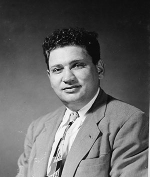
This tiny post is devoted to a cute reverse Pinsker inequality, extracted from a recent work of my colleague Justin Salez. This reverse Pinsker inequality is at the heart of his investigation of the cutoff phenomenon, in total variation distance, for Markov chains, that we do not discuss here.

Pinsker inequality. If $\mu$ and $\nu$ are probability measures on the same probability space, it reads
$$2\|\mu-\nu\|_{\mathrm{TV}}^2\leq\mathrm{Entropy}(\nu\mid\mu)$$ where
$$\mathrm{Entropy}(\nu\mid\mu):=\int\frac{\mathrm{d}\nu}{\mathrm{d}\mu}\log\frac{\mathrm{d}\nu}{\mathrm{d}\mu}\mathrm{d}\mu.$$ is the Kullback-Leibler divergence or relative entropy of $\nu$ with respect to $\mu$, and where
$$\|\mu-\nu\|_{\mathrm{TV}}:=\sup_A|\mu(A)-\nu(A)|$$ is the total variation distance between $\mu$ and $\nu$. By convention $\mathrm{Entropy}(\nu\mid\mu)=+\infty$ if $\frac{\mathrm{d}\nu}{\mathrm{d}\nu}$ does not exist, and in this case the inequality is useless. The constant $2$ is optimal as one can check on Bernoulli distributions. The inequality was first proved by Mark S. Pinsker (1925 – 2003) with another constant, and later on and independently by Solomon Kullback (1907 – 1994) and Imre Csiszár (1938 – ). Let us give now a quick proof, due to Johannes H. B. Kemperman (1924 – 2011). Using $\|\mathrm{1}_A-\mathrm{1}_{A^c}\|_\infty\leq1$, the $L^1-L^\infty$ duality, the convexity inequality $$3(u-1)^2\leq(2u+4)(u\log u-u+1),\quad u\geq0,$$ and the Cauchy-Schwarz inequality, we get, with $\alpha:=\alpha_{\nu\mid\mu}:=\frac{\mathrm{d}\nu}{\mathrm{d}\mu}$, $$\begin{align*} 2\|\mu-\nu\|_{\mathrm{TV}} &\leq\sup_{\|f\|_\infty\leq1}\int f\mathrm{d}(\mu-\nu)\\ &=\int|\alpha-1|\mathrm{d}\mu\\ &\leq\int\sqrt{\frac{2\alpha+4}{3}}\sqrt{\alpha\log\alpha-\alpha+1}\mathrm{d}\mu\\ &\leq\sqrt{\int\frac{2\alpha+4}{3}\mathrm{d}\mu}\sqrt{\int\alpha\log\alpha\mathrm{d}\mu}\\ &=\sqrt{2\int\alpha\log\alpha\mathrm{d}\mu}\\ &=\sqrt{2\mathrm{Entropy}(\nu\mid\mu)}. \end{align*}$$ Note that $\left\|\cdot\right\|_{\mathrm{TV}}$ takes its values in $[0,1]$ while $\mathrm{Entropy}$ takes its values in $[0,+\infty]$. Indeed if $\mathrm{d}\nu=\frac{\mathrm{1}_A}{\mu(A)}\mathrm{d}\mu$, then $\|\mu-\nu\|_{\mathrm{TV}}=1-\mu(A)$ while $\mathrm{Entropy}(\nu\mid\mu)=-\log\mu(A)\to+\infty$ as $\mu(A)\to0$. Also we cannot expect a direct reverse Pinsker inequality.

Varentropy. The relative entropy can be seen as the mean of a log :
$$\mathrm{Entropy}(\nu\mid\mu)=\int\beta_{\nu\mid\mu}\mathrm{d}\nu \quad\text{where}\quad \beta_{\nu\mid\mu}:=\log\frac{\mathrm{d}\nu}{\mathrm{d}\mu}.$$ The variance of $\beta_{\nu\mid\mu}$ or varentropy is
$$\begin{align*} \mathrm{Varentropy}(\nu\mid\mu) &:= \mathrm{Var}_\nu(\beta_{\nu\mid\mu})\\ &=\int(\beta_{\nu\mid\mu}-\mathrm{Entropy}(\nu\mid\mu))^2\mathrm{d}\nu\\ &=\int\beta_{\nu\mid\mu}^2\mathrm{d}\nu-\mathrm{Entropy}(\nu\mid\mu)^2. \end{align*}$$ If $\mathrm{d}\nu=\frac{\mathrm{1}_A}{\mu(A)}\mathrm{d}\mu$ then $\beta_{\nu\mid\mu}$ is constant on $A=\mathrm{supp}(\nu)$ and $\mathrm{Varentropy}(\nu\mid\mu)=0$.

A reverse Pinsker inequality. It reads
$$\mathrm{Entropy}(\nu\mid\mu) \leq\frac{1+\sqrt{\mathrm{Varentropy}(\nu\mid\mu)}}{1-\|\mu-\nu\|_{\mathrm{TV}}}.$$ In particular for all $\varepsilon\in(0,1)$,
$$\|\mu-\nu\|_{\mathrm{TV}}\leq\varepsilon \quad\Longrightarrow\quad \mathrm{Entropy}(\nu\mid\mu) \leq\frac{1+\sqrt{\mathrm{Varentropy}(\nu\mid\mu)}}{1-\varepsilon}.$$ Let us give a proof. Let us set $\varepsilon:=\|\mu-\nu\|_{\mathrm{TV}}$. Consider the event
$$A:=\Bigr\{\frac{\mathrm{d}\nu}{\mathrm{d}\mu}\geq\mathrm{e}^\theta\Bigr\} \quad\text{where}\quad \theta:=\mathrm{Entropy}(\nu\mid\mu)-\frac{\sqrt{\mathrm{Varentropy}(\nu\mid\mu)}}{1-\varepsilon}.$$ The Chebyshev inequality gives $$\begin{align*} \nu(A^c) &=\nu(\beta_{\nu\mid\mu}<\theta)\\ &=\nu\Bigr(\beta_{\nu\mid\mu}-\mathrm{Entropy}(\nu\mid\mu)<-\frac{\sqrt{\mathrm{Varentropy}(\nu\mid\mu)}}{1-\varepsilon}\Bigr)\\ &\leq(1-\varepsilon)^2, \end{align*}$$ hence $\nu(A)\geq1-(1-\varepsilon)^2$. On the other hand, the definition of $A$ gives
$$\mu(A)\leq\mathrm{e}^{-\theta}\nu(A).$$ These two inequalities together give
$$\nu(A)-\mu(A)\geq(1-(1-\varepsilon)^2)(1-\mathrm{e}^{-\theta}).$$ Now since $\|\mu-\nu\|_{\mathrm{TV}}=\varepsilon$, we get $\varepsilon\geq(1-(1-\varepsilon)^2)(1-\mathrm{e}^{-\theta})$, in other words
$$\theta\leq\log\Bigr(1+\frac{1}{1-\varepsilon}\Bigr).$$ Finally, the convexity inequality $\log(1+u)\leq u$ gives $\theta\leq1/(1-\varepsilon)$, as expected.

If $\mathrm{d}\nu=\frac{\mathrm{1}_A}{\mu(A)}\mathrm{d}\mu$ then the reverse Pinsker inequality above reads $-\mu(A)\log\mu(A)\leq1$.

Fisher information and Poincaré inequality. The logarithmic Fisher information is defined by
$$\mathrm{Fisher}(\nu\mid\mu) :=\int|\nabla\beta_{\nu\mid\mu}|^2\mathrm{d}\nu =\int\frac{|\nabla\frac{\mathrm{d}\nu}{\mathrm{d}\mu}|^2}{\frac{\mathrm{d}\nu}{\mathrm{d}\mu}}\mathrm{d}\mu.$$ Also we have, denoting $c_{\mathrm{PI}}(\nu)$ the Poincaré inequality constant of $\nu$ :
$$\mathrm{Varentropy}(\nu\mid\mu) = \mathrm{Var}_\nu(\beta_{\nu\mid\mu}) \leq c_{\mathrm{PI}}(\nu)\int|\nabla\beta_{\nu\mid\mu}|^2\mathrm{d}\nu =c_{\mathrm{PI}}(\nu)\mathrm{Fisher}(\nu\mid\mu).$$ Combined with the reverse Pinsker inequality above, this gives
$$\mathrm{Entropy}(\nu\mid\mu) \leq\frac{1+\sqrt{c_{\mathrm{PI}}(\nu)\mathrm{Fisher}(\nu\mid\mu)}}{1-\|\mu-\nu\|_{\mathrm{TV}}}.$$

Note. There are plenty of alternate or reverse Pinsker inequalities. For instance the Bretagnolle-Huber inequality, used for hypothesis testing in Statistics, reads $$\|\mu-\nu\|_{\mathrm{TV}}^2\leq1-\mathrm{e}^{-\mathrm{Entropy}(\nu\mid\mu)},$$ and has the advantage over Pinsker of being informative even when $\mathrm{Entropy}(\nu\mid\mu)\geq2$.

Further reading.

• Johannes H. B. Kemperman.
  On the optimum rate of transmitting information (in particular pages 2174-2175)
  Annals of Mathematical Statistics, 40:2156–2177 (1969)
• Justin Salez
  Cutoff for non-negatively curved Markov chains (in particular Lemma 8)
  To appear in Journal of the European Mathematical Society (2023)
  See also arXiv:2102.05597