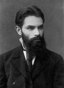
Lindeberg, in his 1922 paper, gave a complete proof of the central limit theorem under more general conditions than Liapunov. He introduced the famous Lindeberg condition of which I shall have more to say below. I was happy to make his personal acquaintance at a mathematical congress in Helsingfors in the summer of 1922. He was Professor at the University of Helsingfors, and owned a beautiful farm in the eastern part of the country. When he was reproached for not being sufficiently active in his scientific work, he said, “Well, I am really a farmer.” And if somebody happened to say that his farm was not properly cultivated, his answer was “Of course, my real job is to be a professor.” I was very fond of him, and saw him often during the following years.
Excerpt from Half a century with probability theory. Some personal recollections, by Harald Cramér (1893 - 1985), published in The Annals of Probability (1976)
The usual proof of the Central Limit Theorem (CLT) served nowadays in courses is based on characteristic functions (Fourier transform). It is attributed essentially to Lyapunov, but was also (re)discovered by others, and extended notably by Lévy. Before him, Chebyshev was using the method of moments! This tiny post is devoted to a less usual yet useful approach by coupling, due to Lindeberg. There are plenty of other approaches, such as the method of (Charles) Stein based on integration by parts, and the method of Linnik based on Shannon information.
Lindeberg replacement or exchange principle, based on coupling.. Let $X_1,\ldots,X_n$ be independent real random variables with with $\mathbb{E}(|X_k|^3)<\infty$. Set $$m_k:=\mathbb{E}(X_k),\quad\sigma^2_k:=\mathbb{E}(|X_k-m_k|^2),\quad\tau_k^3:=\mathbb{E}(|X_k-m_k|^3).$$Let $Y_1,\ldots,Y_n$ be independent, and independent of $X_1,\ldots,X_n$, such that $$Y_k\sim\mathcal{N}(m_k,\sigma^2_k).$$Then for all $f\in\mathcal{C}^3(\mathbb{R},\mathbb{R})$ with $f,f',f'',f^{(3)}$ bounded,$$|\mathbb{E}(f(X_1+\cdots+X_n))-\mathbb{E}(f(Y_1+\cdots+Y_n))|\leq(\tau_1^3+\cdots+\tau_n^3)\frac{{\|f^{(3)}\|}_\infty}{2}.$$This Lindeberg coupling inequality implies immediately that if $$S_n:=\frac{X_1-m_1+\cdots+X_n-m_n}{\sqrt{\sigma_1^2+\cdots+\sigma_n^2}}\quad\text{and}\quad G\sim\mathcal{N}(0,1)$$ then for all $f\in\mathcal{C}^3(\mathbb{R},\mathbb{R})$ with $f,f',f'',f^{(3)}$ bounded, $$|\mathbb{E}(f(S_n))-\mathbb{E}(f(G))|\leq\frac{\tau_1^3+\cdots+\tau_n^3}{\sqrt{\sigma_1^2+\cdots+\sigma_n^2}^3}\frac{{\|f^{(3)}\|}_\infty}{2}.$$In the iid case, $m_k$, $\sigma_k$, and $\tau_k$ no longer depend on $k$, and $$\frac{\tau_1^3+\cdots+\tau_n^3}{\sqrt{\sigma_1^2+\cdots+\sigma_n^2}^3}=\frac{\tau^3}{\sigma^3\sqrt{n}}.$$We thus get a quantitative (non-asymptotic) version of the CLT, in the spirit of the Berry-Esseen inequality. In terms of asymptotic analysis, this also leads to the classical iid CLT under finite third moment by approximating indicators by smooth functions, namely, for all $x\in\mathbb{R}$, $\varepsilon>0$, there exists $f,g\in\mathcal{C}^3(\mathbb{R},\mathbb{R})$ with $f,f',f'',f^{(3)},g,g',g'',g^{(3)}$ bounded such that $$\mathbf{1}_{(-\infty,x-\varepsilon]}\leq f_\varepsilon\leq\mathbf{1}_{(-\infty,x]}\leq g_\varepsilon\leq\mathbf{1}_{(-\infty,x+\varepsilon]}.$$
Let us prove the Lindeberg coupling inequality above. Since the statement is invariant by translation on $f$, we can assume without loss of generality that $m_k=0$ for all $k$. The idea now is to replace, in $X_1+\cdots+X_n$, $X_k$ by $Y_k$, step by step. Namely, introducing $$Z_k:=X_1+\cdots+X_{k-1}+Y_{k+1}\cdots+Y_n,$$we get the telescopic sum $$f(X_1+\cdots+X_n)-f(Y_1+\cdots+Y_n)=\sum_{k=1}^n(f(Z_k+X_k)-f(Z_k+Y_k)).$$Now, the Taylor-Lagrange formula applied at $Z_k$ at order $2$ gives $$f(Z_k+X_k)=f(Z_k)+f'(Z_k)X_k+f''(Z_k)\frac{X_k^2}{2!}+f^{(3)}(Z_k)\frac{A_k^3}{3!}$$where $A_k\in[Z_k,Z_k+X_k]$. Similarly, $$f(Z_k+Y_k)=f(Z_k)+f'(Z_k)Y_k+f''(Z_k)\frac{Y_k^2}{2!}+f^{(3)}(Z_k)\frac{B_k^3}{3!}$$ where $B_k\in[Z_k,Z_k+Y_k]$. Taking the expectation, using the independence of $(X_k,Y_k)$ and $Z_k$, and using the fact that the first two moments of the $X_k$'s and the $Y_k$'s match, we get $$|f(Z_k+X_k)-f(Z_k+Y_k)|\leq\frac{{\|f^{(3)}\|}_\infty}{3!}\mathbb{E}(|X_k|^3+|Y_k|^3).$$ It remains to note that $Y_k=\sigma(X_k)G_k$ where $G_k\sim\mathcal{N}(0,1)$, hence $$\mathbb{E}(|Y_k|^3)=\mathbb{E}(|X_k|^2)^{3/2}\mathbb{E}(|G_k|^3)\leq2\mathbb{E}(|X_k|^3).$$
Lindeberg second moment truncation condition. It should not be confused with the Lindeberg replacement principle above. More precisely, for sums of independent square integrable random variables, beyond the finite third moment condition, the CLT holds as soon as the Lindeberg second moment truncation condition holds: for all $\varepsilon>0$, $$\lim_{n\to\infty}\frac{1}{\sigma_1^2+\cdots+\sigma_n^2}\sum_{k=1}^n\mathbb{E}((X_k-m_k)^2\mathbf{1}_{\{|X_k-m_k|\geq\varepsilon\sigma_k\}})=0.$$ This holds in particular if the Lyapunov moment condition is satisfied: for some $p>1$, $$\lim_{n\to\infty}\frac{1}{{(\sigma_1^2+\cdots+\sigma_n^2)}^{p}}\sum_{k=1}^n\mathbb{E}(|X_k-m_k|^{2p})=0,$$as we can check using the Markov inequality $\mathbf{1}_{\{|X_k-m_k|\geq\varepsilon\sigma_k\}}\leq\frac{|X_k-m_k|}{\varepsilon\sigma_k}$. These versions of the CLT for sums of independent variables extend to martingales. Lindeberg's work on the CLT was reinvented independently by Alan Turing in his dissertation on the central limit theorem!
Comments. The replacement principle can be used beyond the realm of sums of independent variables, typically for nonlinear stochastic models involving independent ingredients, for instance for the high dimensional asymptotic analysis of the eigenvalues of random matrices.
Je regardai d'abord les livres classiques de Joseph Bertrand, de Poincaré, et d'Émile Borel. Seul Poincaré avait esquissé une tentative de justification de la loi de Gauss; mais ce n'était qu'une esquisse. ... II fallait me mettre à la tâche, ce que je fis. Mais je devais avoir des déceptions ; je ne devais d'abord que redécouvrir des résultats déjà obtenus en Russie par Tchebichev et Liapounov. Mais, avant de parler des erreurs expérimentales, il fallait parler des principes du calcul des probabilités. Je m'aperçus alors qu'en un certain sens ce calcul n'existait pas ; il fallait le créer (note: more than ten years before Kolmogorov 1933).
Excerpt from Quelques aspects de la pensée d'un mathématicien, by Paul Lévy (1886 - 1971), published by Librairie Armand Blanchard (1970)
« Cette loi ne s'obtient pas par des déductions rigoureuses ; plus d’une démonstration qu’on a voulu en donner est grossière, entre autres celle qui s’appuie sur l’affirmation que la probabilité des écarts est proportionnelle aux écarts. Tout le monde y croit cependant, me disait un jour M. Lippmann, car les expérimentateurs s’imaginent que c’est un théorème de mathématiques, et les mathématiciens que c’est un fait expérimental. »
Excerpt from Le calcul des Probabilités (1896), by Henri Poincaré (1854 - 1912), about the normal law and the CLT known at that time as « loi des erreurs ». Quoting the catalan physicist Oriol Bohigas (1925 - 2021), « de nos jours, nous savons que c'est à la fois un fait expérimental et un théorème de mathématiques !».
Further reading.
- Cramér, Harald
Half a century with probability theory. Some personal recollections.
The Annals of Probability (1976) - Aldrich, John
England and Probability in the Inter-War Years
Electronic Journal for History of Probability and Statistics (2009) - Lévy, Paul
Quelques aspects de la pensée d'un mathématicien
Librairie Albert Blanchard (1970) - Lindeberg, Jarl Waldemar
Eine neue Herleitung des Exponentialgesetzes in der Wahrscheinlichkeitsrechnung
Mathematische Zeitschrift (1922) - Hans Fischer
A History of the Central Limit Theorem - From Classical to Modern Probability Theory
Springer (2011) - Feller, William
An Introduction to Probability Theory and Its Applications
Wiley (1968) - Billingsley, Patrick
Probability and Measure
Wiley (1995) - Chatterjee, Sourav
A generalization of the Lindeberg principle
Annals of Probability (2006) - Tao, Terence
Least singular value, circular law, and Lindeberg exchange
Random matrices, American Mathematical Society (2019) - On this blog
When the central limit theorem fails… Sparsity and localization (2010)