This post is about a link between large deviations inequalities and the central limit phenomenon. In a nutshell, for the random walk $S_n:=X_1+\cdots+X_n$ where $X_1,\ldots,X_n$ are independent copies on a real random variables $X$, the Markov inequality yields, for all $x$,
$$
\mathbb{P}\Bigr(\frac{S_n}{n}\geq x\Bigr)
\overset{\lambda>0}{=}
\mathbb{P}(\mathrm{e}^{\lambda S_n}\geq\mathrm{e}^{n\lambda x})
\leq\mathrm{e}^{-n\sup_{\lambda\geq0}(\lambda x-\log\mathbb{E}(\mathrm{e}^{\lambda X}))}.
$$ The variational function of $x$ in the right hand side reminds the Legendre transform of the log-Laplace transform, known as the Cramér transform. When $X$ has finite exponential moments, we obtain, for $x=\mathbb{E}(X)+r$, a reinforcement of the law of large numbers in terms of an exponential deviation inequality for $\frac{S_n}{n}$ from $\mathbb{E}(X)$. This leads to the Cramér large deviations principle. When $x=\mathbb{E}(X)+\frac{r}{\sqrt{n}}$, the left hand side is at the CLT scale and the right hand side leads to the second derivative, at $\mathbb{E}(X)$, of the Cramér transform, which turns out to be $\frac{1}{\mathrm{Var}(X)}$, making the upper bound Gaussian in accordance with the CLT.
Legendre transform. Let us consider a function
$$
\Phi:\mathbb{R}\to(-\infty,+\infty].
$$ We assume that $\Phi\not\equiv+\infty$, namely that
$$
\{\lambda\in\mathbb{R}:\Phi(\lambda)<+\infty\}\neq\varnothing.
$$ Then its Legendre transform $\Phi^*:\mathbb{R}\to(-\infty,+\infty]$ is defined for all $x\in\mathbb{R}$ by
$$
\Phi^*(x):=\sup_{\lambda\in\mathbb{R}}(\lambda x-\Phi(\lambda))
=\sup_{\Phi(\lambda) < +\infty}(\lambda x-\Phi(\lambda)).
$$ Since $\Phi^*$ is the envelope of a family of affine functions, it is convex. Famous examples :
$$
\begin{array}{c|c|c|c}
\Phi(\lambda) & \{\Phi<+\infty\} & \Phi^*(x) & \{\Phi^*<+\infty\}\\\hline
|\lambda|^p, 1 < p < \infty & \mathbb{R} & |x|^q, \frac{1}{p}+\frac{1}{q}=1 & \mathbb{R}\\
|\lambda| & \mathbb{R} & 0 & [-1,1] \\
\mathrm{e}^\lambda & \mathbb{R} & x\log(x)-x & [0,+\infty)
\end{array}
$$ For all $\lambda$ and $x$, the definition of $\Phi^*$ gives the Young or Fenchel inequality :
$$
\Phi(\lambda)+\Phi^*(x)\geq\Phi(\lambda)+\lambda x-\Phi(\lambda)=\lambda x.
$$ If $\Phi$ is convex, differentiable on an open interval $I\subset\{\Phi<+\infty\}$ with $\Phi'$ injective, then $\Phi^*$ is differentiable on $\Phi'(I)$ and satisfies the Legendre fundamental relation :
$$
(\Phi^*)'=(\Phi')^{-1}.
$$ Indeed, under these assumptions on $\Phi$ the function $\lambda\mapsto\lambda x-\Phi(\lambda)$ is then concave and achieves its supremum at $\lambda=(\Phi')^{-1}(x)$, hence the Legendre formula
$$
\Phi^*(x)=
x(\Phi')^{-1}(x)-\Phi((\Phi')^{-1}(x)),
$$ which shows that $\Phi^*$ is differentiable and gives
$$
(\Phi^*)'(x)
=(\Phi')^{-1}(x)+x((\Phi')^{-1})'(x)-\Phi'((\Phi')^{-1}(x))((\Phi')^{-1})'(x)
=(\Phi')^{-1}(x).
$$ If $\Phi^*\not\equiv+\infty$ then $\Phi^{**}:\mathbb{R}\to(-\infty,+\infty]$ is well defined, the Young inequality gives $\Phi\geq\Phi^{**}$, and $\Phi^{**}$ appears as a convexification of $\Phi$. The Legendre fundamental relation indicates that $\Phi^{**}=\Phi$ if $\Phi$ is convex, and $\Phi$ and $\Phi^*$ are then the Legendre transform of each other : we say that they are conjugate convex functions, and we speak about convex duality.
The Legendre transform is a fundamental tool in nonlinear analysis due to its deep link with convexity. In classical mechanics, it relates the Lagrangian with the Hamiltonian, in thermodynamics and in statistical physics, it relates important variables and in particular the free energy is a Legendre transform. In information theory and in statistics, the Kullback-Leibler relative entropy is the Legendre transform of the log-Laplace transform. In probability theory, the Cramér large deviations principle involves the Legendre transform of the logarithm of the Laplace transform. A take home idea is that if a problem involves a function which is convex in a variable, it is often interesting to consider its Legendre transform, which corresponds to a remarkably structured nonlinear change of variable and duality.
Cramér transform. The Laplace transform of a real random variable $X$ is given for all $\lambda\in\mathbb{R}$ by
$$
L(\lambda):=\mathbb{E}(\mathrm{e}^{\lambda X})\in[0,+\infty].
$$ If it is finite in a neighborhood of $0$, then for all $n\geq0$, by dominated convergence,
$$
L^{(n)}(\lambda)=\mathbb{E}(X^n\mathrm{e}^{\lambda X})
$$ in other words $L$ is the moments generating function :
$$
L(\lambda)=\sum_{n=0}^\infty\frac{\mathbb{E}(X^n)}{n!}\lambda^n,
\quad\text{in particular}\ L(0)=1,\ L'(0)=\mathbb{E}(X),\ L''(0)=\mathbb{E}(X^2).
$$ The logarithm of the Laplace transform, or log-Laplace transform, is
$$
\Lambda(\lambda):=\log L(\lambda)\in(-\infty,+\infty].
$$ It is the cumulants generating function. We have
$$
\Lambda'(\lambda)=\frac{L'(\lambda)}{L(\lambda)}=\frac{\mathbb{E}(X\mathrm{e}^{\lambda X})}{L(\lambda)}
\quad\text{and}\quad
\Lambda''(\lambda)=\frac{\mathbb{E}(X^2\mathrm{e}^{\lambda X})L(\lambda)-\mathbb{E}(X\mathrm{e}^{\lambda X})^2}{L(\lambda)^2}.
$$ In particular
$$
\Lambda(0)=0,\quad
\Lambda'(0)=\mathbb{E}(X),\quad
\Lambda''(0)=\mathbb{E}(X^2)-\mathbb{E}(X)^2=\mathrm{Var}(X).
$$ The log-Laplace transform $\Lambda$ is convex, indeed the Hölder inequality for $p=1/\theta$ gives
$$
\Lambda(\theta\lambda_1+(1-\theta)\lambda_2)
=\log\mathbb{E}((\mathrm{e}^{\lambda_1 X})^\theta(\mathrm{e}^{\lambda_2 X})^{1-\theta})
\leq\theta\Lambda(\lambda_1)+(1-\theta)\Lambda(\lambda_2).
$$ The Cramér transform is the Lengendre transform of the log-Laplace transform :
$$
\Lambda^*(x):=\sup_{\lambda\in\mathbb{R}}(\lambda x-\Lambda(\lambda)).
$$ Since $\Lambda^*(x)\geq 0x-\Lambda(0)=0$ for all $x\in\mathbb{R}$, we always have
$$
\Lambda^*\geq0.
$$ Examples of Cramér transforms :
\begin{array}{c|c|c}
\text{Distribution}
& \Lambda(\lambda)
& \Lambda^*(x)\\\hline
\underset{\text{Bernoulli}\ 0 < p < 1}{p\delta_1+(1-p)\delta_0} & \log(p\mathrm{e}^{\lambda}+(1-p)) & \begin{cases} x\log\frac{x}{p}+(1-x)\log\frac{1-x}{1-p}&\text{if $x\in[0,1]$}\\ +\infty&\text{otherwise} \end{cases}\\ \underset{\text{Poisson}\ \theta>0}{\mathrm{e}^{-\theta}\sum_{n=0}^\infty\frac{\theta^n}{n!}\delta_n}
&\theta(\mathrm{e}^{\lambda}-1)
&\begin{cases}
\theta-x+x\log\frac{x}{\theta}&\text{if $x\geq0$}\\
+\infty&\text{otherwise}
\end{cases}\\
\underset{\text{Exponential}\ \theta>0}{\theta\mathrm{e}^{-\theta x}\mathbb{1}_{x\geq0}\mathrm{d}x}
&\begin{cases}
\log\frac{\theta}{\theta-\lambda}&\text{if $\lambda<\theta$}\\ +\infty&\text{otherwise} \end{cases} &\begin{cases} \theta x-1-\log(\theta x)&\text{if $x>0$}\\
+\infty&\text{otherwise}
\end{cases}\\
\underset{\text{Gaussian}\ m\in\mathbb{R},\ \sigma>0}{\frac{1}{\sqrt{2\pi\sigma^2}}\mathrm{e}^{-\frac{(x-m)^2}{2\sigma^2}}\mathrm{d}x}
&\lambda m+\frac{\sigma^2}{2}\lambda^2
&\frac{(x-m)^2}{2\sigma^2}
\end{array}
In these examples, $\Lambda$ is finite in a neighborhood of $0$ with $\Lambda''>0$. Under these conditions, $X$ has all its moments finite, and remembering the properties of the Legendre transform, we get $\Lambda'(0)=\mathbb{E}(X)$ which gives $(\Lambda')^{-1}(\mathbb{E}(X))=0$, $\Lambda''(0)=\mathrm{Var}(X)>0$, and
$$
(\Lambda^*)''(\mathbb{E}(X))
=((\Lambda')^{-1})'(\mathbb{E}(X))
=\frac{1}{\Lambda''((\Lambda')^{-1}(\mathbb{E}(X)))}
=\frac{1}{\Lambda''(0)}
=\frac{1}{\mathrm{Var}(X)}.
$$ The function $\Lambda^*$ vanishes at its unique minimizer $\mathbb{E}(X)$. Moreover, if $x\geq\mathbb{E}(X)$, then
$$
\Lambda^*(x)=\sup_{\lambda\geq0}(\lambda x-\Lambda(\lambda)).
$$ Indeed, if $x\geq\mathbb{E}(X)$ and $\lambda\leq0$ then $x\lambda-\Lambda(\lambda)\leq x\mathbb{E}(X)-\Lambda(\lambda)\leq0$ by the Jensen inequality, while $\Lambda^*(x)\geq0$ always. Similarly, if $x\leq\mathbb{E}(X)$, then
$$
\Lambda^*(x)=\sup_{\lambda\leq0}(\lambda x-\Lambda(\lambda)).
$$
Cramér-Chernoff large deviation upper bound. With all the above we get, for all $x\in\mathbb{R}$,
$$
\mathbb{P}\Bigr(\frac{S_n}{n}\geq x\Bigr)
\leq\exp\Bigr(-n\Lambda^*(x)\Bigr).
$$ It follows that for all $r\geq0$,
$$
\mathbb{P}\Bigr(\sqrt{n}\Bigr(\frac{S_n}{n}-\mathbb{E}(X)\Bigr)\geq r\Bigr)
\leq\exp\Bigr(-n\Lambda^*\Bigr(\mathbb{E}(X)+\frac{r}{\sqrt{n}}\Bigr)\Bigr).
$$ Now, since $\Lambda^*(\mathbb{E}(X))=(\Lambda^*)'(\mathbb{E}(X))=0$, $(\Lambda^*)''(\mathbb{E}(X))=\frac{1}{\mathrm{Var}(X)}$, by a Taylor formula,
$$
\Lambda^*\Bigr(\mathbb{E}(X)+h\Bigr)
=\frac{h^2}{2}(\Lambda^*)''(\mathbb{E}(X))+o(h^2)
=\frac{h^2}{2\mathrm{Var}(X)}+o(h^2),
$$ and we get finally the Gaussian estimate
$$
\mathbb{P}\Bigr(\sqrt{n}\Bigr(\frac{S_n}{n}-\mathbb{E}(X)\Bigr)\geq r\Bigr)
\leq\exp\Bigr(-\frac{r^2}{2\mathrm{Var}(X)}+o_{n\to\infty}(1)\Bigr).
$$ Beyond the model of the empirical mean for iid samples, this suggests a way to pass from a large deviations principle (LDP) to a central limit theorem (CLT). The take home message is that up to regularity aspects, the second order derivative of the LDP rate functional at its minimizer gives the variance of a CLT. When this second order derivative vanishes, the CLT may still hold but at another scale (as for the critical Curie-Weiss model for example). The method applies to most large deviations principles for Boltzmann-Gibbs measures describing interacting particle systems. The classical example in statistical mechanics is the magnetization for the Curie-Weiss model. Another example in statistical physics is the linear statistics for Riesz gases including Coulomb gases. More precisely, in that case, the rate function is the infinite dimensional quadratic form
$$
\mathrm{I}(\mu)=\frac{1}{2}\iint K(x-y)\mathrm{d}\mu(x)\mathrm{d}\mu(y)+\int V(x)\mathrm{d}\mu(x)
$$ for which the second derivative is constant and equal to the kernel $K$, which is, for Coulomb gases, the inverse Laplacian $-c_d\Delta^{-1}$, hence the link with the Gaussian Free Field (GFF). A way to make this rigorous is to extract from the LDP an asymptotic analysis for the log-Laplace of the object of interest for the CLT. For Coulomb gazes, this is done via loop equations.
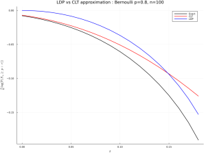
Numerical experiment with Julia.

using Distributions, LaTeXStrings, Plots, Printf
# using Pkg; Pkg.add.(["Distributions", "LaTeXStrings", "Plots", "Printf"])
n = 100 ; p = .8 ; q = 1-p ; dx = .01 ; r = collect(0:dx:1-p-dx) ; x = r.+p
exa = Distributions.ccdf.(Binomial(n,p),n*x)
clt = Distributions.ccdf.(Normal(n*p,sqrt(n*p*q)),n*x)
ldp = exp.(-n.*(x.*log.(x./p)+(1 .-x).*log.((1 .-x)./q)))
plot(r,log.(exa)./n,color=[:black],lw=2,label="Exact")
plot!(r,log.(clt)./n,color=[:red],lw=2,label="CLT")
plot!(r,log.(ldp)./n,color=[:blue],lw=2,label="LDP")
title!(@sprintf("LDP vs CLT approximation : Bernoulli p=%2.1f, n=%d",p,n))
xlabel!("r") ; ylabel!(L"\frac{1}{n}\log(\mathbb{P}(S_n\geq p+r))") ;
plot!(size=(1024,768)); savefig("ldp-clt-ber.png") ; gui()
Further reading.
- Wlodzimierz Bryc
A remark on the connection between the large deviation principle and the central limit theorem
Statistics & Probability Letters 18 253-256 (1993) - Frank den Hollander
Large deviations - specifically Section I.4(7)
Fields Institute Monographs 14 - American Mathematical Society (2000) - Gérard Ben Arous and Marc Brunaud
The Laplace method: variational study of the fluctuations of mean-field diffusions
Stochastics Stochastics Reports 31(1-4) 79–144 (1990) - Djalil Chafaï
Aspects of Coulomb gases - specifically Section 5
Panoramas et Synthèses 59 - Société Mathématique de France, 1–40 (2023) - Michèle Audin et Jean-Pierre Kahane
Portrait d'Adrien-Marie Legendre (1752 - 1833) ?
Image des mathématiques, 8 mai 2011