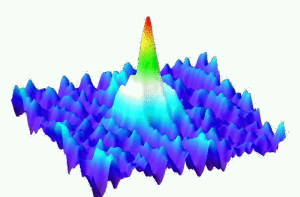
In quantum mechanics, the spin-statistics theorem states that sub-atomic particles are either bosons or fermions. Photons are bosons, while electrons are fermions. Bosons have integer spin, and the wave function of a system of two bosons is symmetric. Fermions have half integer spin, and the wave function of a system of two fermions is antisymmetric. Bosons can occupy the same quantum state, and obey to the Bose-Einstein statistics. Fermions cannot occupy the same quantum state (Pauli exclusion principle), and obey to the Fermi-Dirac statistics. These statistics can be retained using some elementary combinatorics, in the spirit of the famous Maxwell-Boltzmann statistics.
Maxwell-Boltzmann statistics. We have \( {m} \) energy levels \( {E_1,\ldots,E_m} \) and \( {n} \) distinguishable particles. If \( {n_i} \) is the number of \( {E_i} \) particles then \( {n=n_1+\cdots+n_m} \) and the average energy of configuration \( {(n_1,\ldots,n_m)} \) is \( {E=n_1E_1+\cdots+n_mE_m} \). There are
\[ \binom{n}{n_1,\ldots,n_m}=n!\prod_{i=1}^m\frac{1}{n_i!} \]
ways to obtain the configuration \( {(n_1,\ldots,n_m)} \) (multinomial coefficient: throw \( {n} \) distinguishable balls into \( {m} \) boxes). In order to get an additive measurement of the degree of freedom, we may take the logarithm. The additive degree of freedom per particle is then \( {\frac{1}{n}\log\binom{n}{n_1,\ldots,n_m}} \). Now, if \( {n\rightarrow\infty} \) with \( {n_i/n\rightarrow p_i} \) for every \( {1\leq i\leq n} \) then \( {p_1+\cdots+p_m=1} \), and thanks to the Stirling formula, the asymptotic degree of freedom per particle is given by
\[ -\sum_{i=1}^mp_i\log(p_i). \]
This quantity is known as the Boltzmann entropy. Maximizing this entropy subject to the fixed average energy constraint \( {E=\sum_{i=1}^mp_iE_i} \) gives
\[ p_i=Z^{-1}e^{-\beta E_i} \]
where the Lagrange multiplier \( {\beta>0} \) can be interpreted to be proportional to an inverse temperature, and were \( {Z=\sum_{i=1}^me^{-\beta E_i}} \) is a normalizing factor.
As pointed out by Gibbs, the reasoning above is faulty. Namely, if we consider a system formed by \( {n+n'} \) particles, then the logarithmic degree of freedom is actually not additive, violating the second principle of thermodynamics. A way to solve this paradox is to assume that the particles are undistinguishable. This makes the combinatorics trivial since for every configuration \( {(n_1,\ldots,n_m)} \) there is a unique way to throw our undistinguishable particles into the \( {m} \) boxes with \( {n_i} \) particles in each box for every \( {1\leq i\leq m} \). To escape from this triviality, we assume that each energy level \( {E_i} \) has \( {s_i} \) states, in other words that box \( {i} \) has \( {s_i} \) sub-boxes. The number of ways to obtain configuration \( {(n_1,\ldots,n_m)} \) is then
\[ \prod_{i=1}^m\frac{(n_i+s_i-1)!}{n_i!(s_i-1)!}. \]
If \( {s_1=\cdots=s_m=1} \) then this number is \( {1} \). If \( {n_i\ll s_i} \) then thanks to the Stirling formula, the number of ways to obtain configuration \( {(n_1,\ldots,n_m)} \) is
\[ \approx\prod_{i=1}^m\frac{s_i^{n_i}}{n_i!}. \]
The variational reasoning used for the distinguishable case leads then to another distribution for the energy levels, known as the Maxwell-Boltzmann statistics:
\[ p_i\approx Z^{-1}s_ie^{-\beta E_i}. \]
When \( {s_1=\cdots=s_m} \) we recover the same distribution.
Bose-Einstein statistics. We follow the reasoning used for the Maxwell-Boltzmann statistics, without the assumption \( {n_i\ll s_i} \). This leads to
\[ p_i\approx Z^{-1}\frac{s_i}{e^{\beta E_i-\alpha}-1}. \]
Fermi-Dirac statistics. Suppose this time that at most one particle can occupy a state (i.e. a sub-box). The number of ways to obtain configuration \( {(n_1,\ldots,n_m)} \) is this time
\[ \prod_{i=1}^m\frac{s_i!}{n_i!(s_i-n_i)!}, \]
leading to
\[ p_i\approx Z^{-1}\frac{s_i}{e^{\beta E_i-\alpha}+1}. \]
Leave a Comment