The Sinkhorn factorization of a square matrix $A$ with positive entries takes the form $$A = D_1 S D_2$$ where $D_1$ and $D_2$ are diagonal matrices with positive diagonal entries and where $S$ is a doubly stochastic matrix meaning that it has entries in $[0,1]$ and each row and column sums up to one. It is named after Richard Dennis Sinkhorn (1934 – 1995) who worked on the subject in the 1960s. A natural algorithm for the numerical approximation of this factorization consists in iteratively normalize each row and each column, and this is referred to as the Sinkhorn-Knopp algorithm. Its convergence is fast. Actually this is a special case of the iterative proportional fitting (IPF) algorithm, classic in probability and statistics, which goes back at least to the analysis of the contingency tables in the 1920s, and which was reinvented many times, see for instance the article by Friedrich Pukelsheim and references therein. It is in particular well known that $S$ is the projection of $A$, with respect to the Kullback-Leibler divergence, on the set of doubly stochastic matrices (Birkhoff polytope). The Sinkhorn factorization and its algorithm became fashionable in the domain of computational optimal transportation due to a relation with entropic regularization. It is also considered in the domain of quantum information theory.
Here is a simple implementation using the Julia programming language.
using LinearAlgebra # for Diagonal
#
function sinkhorn(A, tol = 1E-6, maxiter = 1E6)
 # Sinkhorn factorization A = D1 S D2 where D1 and D2 are diagonal and S doubly
 # stochastic using Sinkhorn-Knopp algorithm which consists in iterative rows
 # and columns sums normalizations. This code is not optimized.
 m , n = size(A,1), size(A,2)
 D1, D2 = ones(1,n), ones(1,n)
 S = A
 iter, err = 0, +Inf
 while ((err > tol) && (iter < maxiter))
   RS = vec(sum(S, dims = 2)) # column vector of rows sums
   D1 = D1 .* RS
   S = Diagonal(1 ./ RS) * S
   CS = vec(sum(S, dims = 1)) # row vector of columns sums
   D2 = CS .* D2
   S = S * Diagonal(1 ./ CS)
   iter += 1
   err = norm(RS .- 1) + norm(CS .- 1)
 end
 return S, Diagonal(D1), Diagonal(D2), iter
end # function
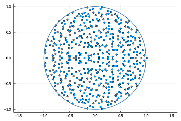
Circular law. Suppose now that $A$ is a random matrix, $n\times n$, with independent and identically distributed positive entries of mean $m$ and variance $\sigma^2$, for instance following the uniform or the exponential distribution. Let $S$ be the random doubly stochastic matrix provided by the Sinkhorn factorization. It is tempting to conjecture that the empirical spectral distribution of $$\frac{m\sqrt{n}}{\sigma}S$$ converges weakly as $n\to\infty$ to the uniform distribution on the unit disc of the complex plane, with a single outlier equal to $\frac{m\sqrt{n}}{\sigma}$. The circular law for $S$ is inherited from the circular law for $A$ and the law of large numbers. This can be easily guessed from the first iteration of the Sinkhorn-Knopp algorithm, that reminds the circular law analysis of random Markov matrices inspired from the Dirichlet Markov Ensemble and its decomposition. The circular law for $A$ is a universal high dimensional phenomenon that holds as soon as the variance of the entries is finite. One can also explore the case of heavy tails, and wonder if the circular law for $S$ still remains true!
The following Julia code produces the graphics at the top and the bottom of this post.
using Printf # for @printf
using Plots # for scatter and plot
using LinearAlgebra # for LinRange

function sinkhornplot(A,m,sigma,filename)
    S, D1, D2, iter = sinkhorn(A)
    @printf("%s\n",filename)
    @printf(" ‖A-D1 S D2‖ = %s\n",norm(A-D1*S*D2))
    @printf(" ‖RowsSums(S)-1‖ = %s\n",norm(sum(S,dims=2).-1))
    @printf(" ‖ColsSums(S)-1‖ = %s\n",norm(sum(S,dims=1).-1))
    @printf(" SK iterations = %d\n",iter)
    spec = eigvals(S) * m * sqrt(size(S,1)) / sigma
    maxval, maxloc = findmax(abs.(spec))
    deleteat!(spec, maxloc)
    scatter(real(spec),imag(spec),aspect_ratio=:equal,legend=false)
    x = LinRange(-1,1,100)
    plot!(x,sqrt.(1 .- x.^2),linewidth=2,linecolor=:steelblue)
    plot!(x,-sqrt.(1 .- x.^2),linewidth=2,linecolor=:steelblue)
    savefig(filename)
end #function

sinkhornplot(rand(500,500),1/2,1/sqrt(12),"sinkhorn-unif.png")
sinkhornplot(-log.(rand(500,500)),1,1,"sinkhorn-expo.png")
sinkhornplot(abs.(randn(500,500)./randn(500,500)),1,1,"sinkhorn-heavy.png")

Example of program output.
sinkhorn-unif.png
 ‖A-D1 S D2‖ = 6.704194265149758e-14
 ‖RowsSums(S)-1‖ = 8.209123420903459e-11
 ‖ColsSums(S)-1‖ = 3.326966272203901e-15
 SK iterations = 4
sinkhorn-expo.png
 ‖A-D1 S D2‖ = 1.9956579227110527e-13
 ‖RowsSums(S)-1‖ = 5.155302149020719e-11
 ‖ColsSums(S)-1‖ = 3.3454392974351074e-15
 SK iterations = 5
sinkhorn-heavy.png
 ‖A-D1 S D2‖ = 8.423054036449791e-10
 ‖RowsSums(S)-1‖ = 4.5152766460217607e-7
 ‖ColsSums(S)-1‖ = 3.8778423131653425e-15
 SK iterations = 126
Further reading.
- Richard Sinkhorn
A relationship between arbitrary positive matrices and doubly stochastic matrices
Ann. Math. Statist. 35:876-879 (1964) - Richard Sinkhorn and Paul Knopp
Concerning nonnegative matrices and doubly stochastic matrices
Pacific J. Math. 21:343-348 (1967) - Friedrich Pukelsheim
Biproportional scaling of matrices and the iterative proportional fitting procedure
Annals of Operations Research 215(1):269-283 (2014) - Julie Champion
Sur les algorithmes de projections en entropie relative avec contraintes marginales
Thèse de doctorat, université de Toulouse (2013) - Djalil Chafaï
The Dirichlet Markov Ensemble
Journal of Multivariate Analysis 101:555-567 (2010) - Charles Bordenave, Pietro Caputo, and Djalil Chafaï
Circular Law Theorem for Random Markov Matrices
Probability Theory and Related Fields 152(3-4):751-779 (2012) - Hoi Nguyen
Random doubly stochastic matrices: the circular law
Ann. Probab. 42(3):1161-1196 (2014)