
This post is the written version of a modest tutorial on Large Deviation Principles (LDP). It was given at ICERM during an inter workshops week of the 2018 Semester Program “Point Configurations in Geometry, Physics and Computer Science” organized notably by Ed Saff, Doug Hardin, and Sylvia Serfaty. I was asked to give such a tutorial by PhD students. The audience was heterogeneous, a mixture of old and young mathematicians from different areas.
Foreword. We speak about large deviation theory or techniques. This set of techniques lies between analysis, probability theory, and mathematical physics. It is strongly connected to classical probabilistic limit theorems, to asymptotic analysis, convex analysis, variational analysis, functional analysis, and to Boltzmann–Gibbs measures. It was developed essentially all along the twentieth century. The indian-american mathematician S. R. S. Varadhan was one of the main investigators and he finally received the Abel Prize in 2007 – and many other prizes – for his work on large deviation techniques. He forged a natural, beautiful, unifying concept covering many dispersed cases, and a set of general techniques to play with it. Personally, if you ask me if I like LDPs I will probably answer
“Show me your rate function first, and I will tell you if I like large deviations!”.
As many other things, an LDP can be beautiful or useful, and can also be ugly or useless. Large deviations techniques are so efficient that they have produced some sort of industry, just like many other techniques in mathematics such as moment methods, etc. Sometimes an LDP provides the best intuitive interpretation of asymptotic phenomena, usually via a physical energy variational principle. This is the case for the convergence to the semicircle distribution of the eigenvalues of high dimensional Gaussian random matrices. The closest basic concept related to LDPs is the Laplace method for the asymptotic behavior of integrals or sums.
There are plenty of classical books about large deviation techniques. Here are two:
- Dembo and Zeitouni – Large deviation techniques and applications. It is quite successful, with more that 1800 citations for the three editions on Mathscinet to date!
- Dupuis and Ellis – A weak convergence approach to the theory of large deviations. Paul Dupuis is professor at Brown University where the ICERM is located.
Here are also two more recent books and a survey oriented towards applications:
- Touchette – The large deviation approach to statistical mechanics;
- den Hollander – Large deviations;
- Rassoul-Agha and Seppäläinen – A course on large deviations with an introduction to Gibbs measures.
Refresh on probabilistic notation. A random variable \( {X} \) is a measurable function defined on a set \( {\Omega} \) equipped with a \( {\sigma} \)-field \( {\mathcal{A}} \) and a probability measure \( {\mathbb{P}} \), and taking values in a state space \( {E} \) equipped with a \( {\sigma} \)-field \( {\mathcal{B}} \). When \( {E} \) is a topological space such as \( {\mathbb{R}} \) then the natural choice for \( {\mathcal{B}} \) is the Borel \( {\sigma} \)-field, while if \( {E} \) is discrete we take for \( {\mathcal{B}} \) the set of subsets of \( {E} \). The law \( {\mu} \) of \( {X} \) is the image measure of \( {\mathbb{P}} \) by \( {X} \). Namely, for all \( {A\in\mathcal{A}} \),
\[ \mu(A) =\mathbb{P}(X^{-1}(A)) =\mathbb{P}(\{\omega\in\Omega:X(\omega)\in A\}) =\mathbb{P}(X\in A). \]
The first and last notations are the ones that we use in practice. For any bounded or positive measurable “test” function \( {f:E\rightarrow\mathbb{R}} \), we have the following transportation or transfer formula that allows to compute the expectation of \( {f(X)} \) using the law \( {\mu} \):
\[ \mathbb{E}(f(X))=\int_\Omega(f\circ X)\mathrm{d}\mathbb{P} =\int_E f\mathrm{d}\mu. \]
Recall also the Markov inequality: if \( {X\geq0} \) is a random variable and \( {x>0} \) a real number, then from \( {x\mathbf{1}_{X\geq x}\leq X} \) we get by taking expectation of both sides that
\[ \mathbb{P}(X\geq x)\leq\frac{\mathbb{E}(X)}{x}. \]
Motivation and Cramér theorem. Let \( {X_1,X_2,\ldots} \) be a sequence of independent and identically distributed real random variables (we say iid) with law \( {\mu} \) and mean \( {m} \). By the law of large number (LLN) we have, almost surely,
\[ S_n=\frac{X_1+\cdots+X_n}{n} \underset{n\rightarrow\infty}{\longrightarrow} m. \]
It follows that if \( {A\subset\mathbb{R}} \) is a Borel set such that \( {m\not\in\overline{A}} \) (closure of \( {A} \)) then
\[ \mathbb{P}(S_n\in A) \underset{n\rightarrow\infty}{\longrightarrow} 0. \]
We would like to understand at which speed this convergence to zero holds. This amounts to the control of large deviations from the mean, literally. More precisely “large deviation techniques” provide an answer which is asymptotically optimal in \( {n} \) at the exponential scale. Let us reveal the basic idea in the case \( {A=[x,\infty)} \) with \( {x>m} \). We force the exponential and we introduce a free parameter \( {\theta>0} \) that we will optimize later on. By Markov’s inequality
\[ \begin{array}{rcl} \mathbb{P}(S_n\in A) &=&\mathbb{P}(S_n\geq x)\\ &=&\mathbb{P}(\theta(X_1+\cdots+X_n)\geq\theta nx)\\ &=&\mathbb{P}(\mathrm{e}^{\theta(X_1+\cdots+X_n)}\geq\mathrm{e}^{\theta nx})\\ &\leq&\mathrm{e}^{-\theta nx}\mathbb{E}(\mathrm{e}^{\theta(X_1+\cdots+X_n)}). \end{array} \]
This requires to assume that the random variables have finite exponential moments, meaning that the Laplace transform \( {\varphi} \) of \( {\mu} \) is well defined and finite:
\[ \theta\in\mathbb{R}\mapsto\varphi(\theta) =\mathbb{E}(\mathrm{e}^{\theta X_1}) =\int\mathrm{e}^{\theta x}\mathrm{d}\mu(x)<\infty. \]
Now since \( {X_1,X_2,\ldots} \) are independent and identically distributed,
\[ \mathbb{E}(\mathrm{e}^{\theta(X_1+\cdots+X_n)}) =\mathbb{E}(\mathrm{e}^{\theta X_1}\cdots\mathrm{e}^{\theta X_n}) =\mathbb{E}(\mathrm{e}^{\theta X_1})\cdots\mathbb{E}(\mathrm{e}^{\theta X_n}) =\varphi(\theta)^n, \]
which gives
\[ \mathbb{P}(S_n\geq r) \leq\mathrm{e}^{-n\left(\theta x-\log\varphi(\theta)\right)}. \]
Since \( {\theta>0} \) is arbitrary we can optimize over it to get
\[ \mathbb{P}(S_n\geq x) \leq\inf_{\theta>0}\mathrm{e}^{-n\left(\theta x-\log\varphi(\theta)\right)} \leq\mathrm{e}^{-n\sup_{\theta>0}\left(\theta x-\log\varphi(\theta)\right)}. \]
An analysis reveals that since \( {x\geq m} \) we have
\[ \mathbb{P}(S_n\geq x) \leq\mathrm{e}^{-n\Phi(x)} \]
where
\[ \Phi(x)=\sup_{\theta\in\mathbb{R}}\left(\theta x-\log\varphi(\theta)\right). \]
The function \( {\Phi} \) is called the Cramér transform of \( {\mu} \). It is the Legendre transform of the logarithm of the Laplace transform of \( {\mu} \). It can be checked that it is convex and lower semi-continuous with compact level sets, and that \( {m} \) is its unique minimizer, and that \( {\Phi(m)=0} \). With a bit more work we get that for any Borel set \( {A\subset\mathbb{R}} \),
\[ \varlimsup_{n\rightarrow\infty} \frac{1}{n}\log\mathbb{P}(S_n\in A) \leq -\inf_{\overline{A}}\Phi. \]
This upper bound in meaningful when \( {m\not\in\overline A} \) and is trivial otherwise since \( {\Phi(m)=0} \). In fact, this upper bound is tight. Indeed essentially Cramér (\( {\approx} \) 1938) and generally Chernoff (\( {\approx} \) 1952) have shown what we call the Cramér theorem:
\[ \mathbb{P}(S_n\in A) \underset{n\rightarrow\infty}{\approx} \mathrm{e}^{-n\inf_A\Phi} \]
in the sense that in addition to the upper bound the following lower bound holds:
\[ \varliminf_{n\rightarrow\infty} \frac{1}{n}\log\mathbb{P}(S_n\in A) \geq -\inf_{\overset{\circ}{A}}\Phi. \]
The infimum runs over the interior of \( {A} \) this time. Topology plays a role here again. Let us give a rough idea of the proof of the lower bound. We focus on the case where \( {A=(-\delta,\delta)} \) for some \( {\delta>0} \). For all \( {0<\varepsilon<\delta} \), we force the exponential by introducing an arbitrary parameter \( {\eta} \) that we will choose later on, namely
\[ \begin{array}{rcl} \mathbb{P}(S_n\in(-\delta,\delta)) &\geq& \mathbb{P}(S_n\in(-\varepsilon,\varepsilon))\\ &=&\displaystyle\int_{|x_1+\cdots+x_n|<n\varepsilon}\mathrm{d}\mu(x_1)\cdots\mathrm{d}\mu(x_n)\\ &\geq&\displaystyle\mathrm{e}^{-n|\eta|\varepsilon}\int_{|x_1+\cdots+x_n|<n\varepsilon} \mathrm{e}^{(x_1\cdots+x_n)\eta} \mathrm{d}\mu(x_1)\cdots\mathrm{d}\mu(x_n)\\ &=&\displaystyle\mathrm{e}^{-n|\eta|\varepsilon+n\log\varphi(\eta)}\int_{|x_1+\cdots+x_n|<n\varepsilon} \mathrm{d}\widetilde\mu_\eta(x_1)\cdots\mathrm{d}\widetilde{\mu}_\eta(x_n) \end{array} \]
where we have introduced the exponentially shifted probability measure
\[ \mathrm{d}\widetilde\mu_\eta(x) =\mathrm{e}^{\eta x-\log\varphi(\eta)}\mathrm{d}\mu(x). \]
Now if we select \( {\eta} \) in such a way that \( {\widetilde\mu_\eta} \) has zero mean, which turns out to be always possible, then, taking iid random variables \( {\widetilde{X_1},\ldots,\widetilde{X_n}} \) of law \( {\widetilde\mu_\eta} \), the law of large numbers (LLN) gives
\[ \int_{|x_1+\cdots+x_n|<n\varepsilon} \mathrm{d}\widetilde\mu_\eta(x_1)\cdots\mathrm{d}\widetilde{\mu}_\eta(x_n) =\mathbb{P}(\widetilde{X_1}+\cdots+\widetilde{X}_n<n\varepsilon) \underset{n\rightarrow\infty}{\longrightarrow} 1. \]
In fact it can be checked that for such an \( {\eta} \) with have
\[ \log\varphi(\eta)=\inf_{\mathbb{R}}\log\varphi=-\Phi(0). \]
It follows that
\[ \varliminf_{n\rightarrow\infty} \frac{1}{n}\log\mathbb{P}(S_n\in(-\delta,\delta)) \geq-|\eta|\varepsilon+\log\varphi(\eta) =-|\eta|\varepsilon-\Phi(0). \]
Taking the limit \( {\varepsilon\rightarrow0} \) gives finally
\[ \varliminf_{n\rightarrow\infty} \mathbb{P}(S_n\in(-\delta,\delta)) \geq -\Phi(0). \]
This is the germ of the proof of the lower bound. It remains essentially to shift by \( {x} \) to get the lower bound for any ball and then to localize to get it for any open set and then for any Borel set. Note that the upper bound is essentially non-asymptotic and looks like a Chernov deviation inequality while the lower bound is asymptotic and relies here on a weak form of the LLN. Basically, the idea for the upper bound is to use the Markov inequality at the exponential scale, whereas the idea of the lower bound is to tilt the probability measure in order to transform the tail event (or rare event) of interest into a non-tail event. The lower bound is more subtle.
Here is the Cramér transform of some usual discrete and continuous distributions:
- Bernoulli \( {p\delta_0+(1-p)\delta_1} \), \( {0<p<1} \), then \( {\Phi(x)=+\infty} \) if \( {x\not\in[0,1]} \) and otherwise
\[ \Phi(x)=x\log\frac{x}{1-p}+(x-1)\log\frac{p}{x-1}; \]
- Poisson of mean \( {\lambda>0} \), the \( {\Phi(x)=+\infty} \) if \( {x\leq 0} \) and otherwise
\[ \Phi(x)=\lambda-x+x\log\frac{x}{\lambda}; \]
- Exponential of parameter \( {\lambda>0} \), then \( {\Phi(x)=+\infty} \) if \( {x>0} \) and otherwise
\[ \Phi(x)=\lambda x-1-\log(\lambda x); \]
- Gaussian of mean \( {m} \) and variance \( {\sigma^2} \), then for all \( {x\in\mathbb{R}} \),
\[ \Phi(x)=\frac{(x-m)^2}{\sigma^2}. \]
The Cramér theorem remains valid for random vectors in \( {\mathbb{R}^d} \), provided that we use the following natural generalization of the Laplace transform and Legendre (and thus Cramér) transform:
\[ \theta\in\mathbb{R}^d\mapsto \varphi(\theta)=\int\mathrm{e}^{\langle\theta,x\rangle}\mathrm{d}\mu(x) \]
and
\[ x\in\mathbb{R}^d\mapsto \Phi(x)=\sup_{\theta\in\mathbb{R}^d}(\langle\theta,x\rangle-\log\varphi(\theta)). \]
Actually the Cramér theorem remains valid for random variables taking values in possibly infinite dimensional spaces provided that we replace the scalar product by the duality. This is know essentially as the Gärtner-Ellis theorem.
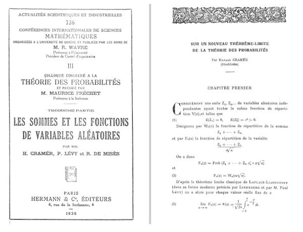
Note. A friend of mine, Arnaud Guyader, brought to my attention that Harald Cramér, who was swedish, published his seminal 1938 paper in French in a conference proceedings with the title Sur un nouveau théorème-limite de la théorie des probabilités. Moreover at the occasion of the 80th anniversary of this paper, Hugo Touchette, who knows very well the subject, translated it in English: arXiv:1802.05988.
Cramér was inspired by Esscher. Here is an excerpt from A conversation with S. R. S. Varadhan by Rajendra Bhatia published in The Mathematical Intelligencer 30 (2008), no. 2, 24-42. Bhatia: “Almost all the reports say that the large-deviation principle starts with Cramér”. Varadhan: “The idea comes from the Scandinavian actuarial scientist Fredrik Esscher. He studied the following problem. An insurance company has several clients and each year they make claims which can be thought of as random variables. The company sets aside certain reserves for meeting the claims. What is the probability that the sum of the claims exceeds the reserve set aside? You can use the central limit theorem and estimate this from the tail of the normal distribution. He found that is not quite accurate. To find a better estimate he introduced what is called tilting the measure (Esscher tilting). The value that you want not to be exceeded is not the mean, it is something far out in the tail. You have to change the measure so that this value becomes the mean and again you can use the central limit theorem. This is the basic idea which was generalized by Cramér. Now the method is called the Cramér transform.”
Varadhan general notion of LDP. The Cramér theorem concerns actually the sequence of probability measures \( {{(\mu_n)}_{n\geq1}} \) where \( {\mu_n} \) is the law of \( {S_n} \). More generally, and following Varadhan, we say that a sequence of probability measures \( {{(\mu_n)}_{n\geq1}} \) on a topological space \( {E} \) equipped with its Borel \( {\sigma} \)-field satisfies a large deviation principle with speed \( {{(a_n)}_{n\geq1}} \) and rate function \( {\Phi} \) when:
- \( {{(a_n)}_{n\geq1}} \) is an increasing sequence of positive reals with \( {\lim_{n\rightarrow\infty}a_n=+\infty} \);
- \( {\Phi:E\rightarrow\mathbb{R}\cup\{\infty\}} \) is a lower semi-continuous function with compact level sets;
- for any Borel subset \( {A\subset E} \), we have \( {\mu_n(A) \underset{n\rightarrow\infty}{\approx} \mathrm{e}^{-a_n\inf_A\Phi}} \) in the sense that
\[ -\inf_{\overset{\circ}{A}}\Phi \leq\varliminf_{n\rightarrow\infty}\frac{\log\mu_n(A)}{a_n} \leq\varlimsup_{n\rightarrow\infty}\frac{\log\mu_n(A)}{a_n} \leq-\inf_{\overline{A}}\Phi. \]
This concept is extraordinarily rich, and the Cramér theorem is an instance of it! It can be shown that the rate function is unique and achieves its infimum on \( {E} \) which is equal to \( {0} \).
Note that this implies by the first Borel-Cantelli lemma that if \( {X_n\sim\mu_n} \) for all \( {n\geq1} \), regardless of the way we construct the joint probability space, then \( {{(X_n)}_{n\geq1}} \) tends almost surely to the set of minimizers \( {\arg\inf} \) of \( {\Phi} \). In many (not all) situations, \( {\Phi} \) turns out to be strictly convex and the minimizer is unique, making the sequence \( {{(X_n)}_{n\geq1}} \) converge almost surely to it. In particular, this observation reveals that the Cramér theorem is stronger than the strong law of large numbers (LLN)!
Contraction principle. This principles states that if a sequence of probability measures \( {{(\mu_n)}_{n\geq1}} \) on a topological space \( {E} \) satisfies to an LDP with speed \( {{(a_n)}_{n\geq1}} \) and rate function \( {\Phi:E\rightarrow\mathbb{R}\cup\{\infty\}} \) then for any continuous \( {f:E\rightarrow F} \), the sequence of probability measures \( {{(\mu_n\circ f^{-1})}_{n\geq1}} \) on \( {F} \) satisfies to an LDP with same speed \( {{(a_n)}_{n\geq1}} \) and rate function (with the convention \( {\inf\varnothing=+\infty} \))
\[ y\in F\mapsto \inf_{f^{-1}(y)}\Phi. \]
This allows to deduce many LDPs from a single LDP.
Laplace-Varadhan and Gibbs principles. The first principle, inspired by the Laplace method and due to Varadhan (\( {\approx} \) 1966) states that if \( {{(\mu_n)}_{n\geq1}} \) is a sequence of probability measures on a topological space \( {E} \) which satisfies to an LDP with speed \( {{(a_n)}_{n\geq1}} \) and rate function \( {\Phi} \) and if \( {f:E\rightarrow\mathbb{R}} \) is say bounded and continuous (this can be weakened) then
\[ \lim_{n\rightarrow\infty}\frac{1}{a_n}\log\int\mathrm{e}^{a_nf}\mathrm{d}\mu_n =\sup_E(\Phi-f). \]
The second principle, due to Ellis (\( {\approx} \) 1985) states that under the same assumptions the sequence of probability measures \( {{(\nu_n)}_{\geq1}} \) defined by
\[ \mathrm{d}\nu_n=\frac{\mathrm{e}^{a_n}f}{\displaystyle\int\mathrm{e}^{a_nf}\mathrm{d}\mu}\mathrm{d}\mu_n \]
satisfies to an LDP with speed \( {{(a_n)}_{n\geq1}} \) and rate function
\[ \Phi-f-\inf_E(\Phi-f). \]
This allows to get LDPs for Gibbs measures when the temperature tends to zero. The measure \( {\nu_n} \) is sometimes called the Esscher transform.
Sanov theorem. My favorite LDP! It was proved essentially by Sanov (\( {\approx} \) 1956) and then by Donsker and Varadhan (\( {\approx} \) 1976). If \( {X_1,X_2,\ldots} \) are independent and identically distributed random variables with common law \( {\mu} \) on a Polish space \( {E} \), then the law of large numbers (LLN) states that almost surely, the empirical measure tends to \( {\mu} \), namely
\[ L_n=\frac{1}{n}\sum_{i=1}^n\delta_{X_i} \underset{n\rightarrow\infty}{\longrightarrow} \mu. \]
This is weak convergence with respect to continuous and bounded test functions. In other words, almost surely, for every bounded and continuous \( {f:E\rightarrow\mathbb{R}} \),
\[ L_n(f)=\frac{1}{n}\sum_{i=1}^nf(X_i) \underset{n\rightarrow\infty}{\longrightarrow} \int f\mathrm{d}\mu. \]
Let \( {\mu_n} \) be the law of the random empirical measure \( {L_n} \) seen as a random variable taking its values in set \( {\mathcal{P}(E)} \) of probability measures on \( {E} \). Then the Sanov theorem states that \( {{(\mu_n)}_{n\geq1}} \) satisfies to an LDP with speed \( {n} \) and rate function given by the relative entropy \( {H(\cdot\mid\mu)} \). In other words, for any Borel subset \( {A\subset\mathcal{P}(E)} \),
\[ \mathbb{P}(L_n\in A)\approx\mathrm{e}^{-n\inf_AH(\cdot\mid\mu)} \]
in the sense that
\[ -\inf_{\overset{\circ}{A}}H(\cdot\mid\mu) \leq\varliminf_{n\rightarrow\infty}\frac{\log\mathbb{P}(L_n\in A)}{n} \leq\varlimsup_{n\rightarrow\infty}\frac{\log\mathbb{P}(L_n\in A)}{n} \leq-\inf_{\overline{A}}H(\cdot\mid\mu). \]
Recall that the relative entropy or Kullback-Leibler divergence is defined by
\[ H(\nu\mid\mu)= \int\frac{\mathrm{d}\nu}{\mathrm{d}\nu}\log\frac{\mathrm{d}\nu}{\mathrm{d}\nu} \mathrm{d}\mu \]
if \( {\nu} \) is aboslutely continuous with respect to \( {\mu} \) and \( {+\infty} \) otherwise. The topology of weak convergence on \( {\mathcal{P}(E)} \) can be metrized with the Bounded-Lipschitz distance
\[ \mathrm{d}_{\mathrm{BL}}(\mu,\nu) =\sup_{\max(\Vert f\Vert_{\infty},\Vert f\Vert_{\mathrm{Lip}})\leq1} \int f\mathrm{d}(\mu-\nu). \]
In particular, by taking \( {A=B(\mu,r)^c} \) for this distance, we can see by the first Borel-Cantelli lemma that almost surely, \( {\lim_{n\rightarrow\infty}L_n=\mu} \) weakly. In other words the Sanov theorem is stronger than the strong law of large numbers (LLN). The theorems of Cramér and Sanov are in fact equivalent in the sense that one can derive one from the other either by taking limits or by discretizing.
Let us give an rough idea of the proof of the upper bound. We recall first the variational formula for the entropy: denoting \( {f=\mathrm{d}\nu/\mathrm{d}\mu} \),
\[ H(\nu\mid\mu) =H_\mu(f) =\sup_{\substack{g\geq0\\\int g\mathrm{d}\mu=1}} \left(\int fg\mathrm{d}\mu-\log\int\mathrm{e}^g\mathrm{d}\mu\right). \]
This formula expresses \( {H} \) as an (infinite dimensional) Legendre transform log the (infinite dimensional) Laplace transform of \( {\mu} \). To establish this variational formula, it suffices to show that \( {t\in[0,1]\mapsto\alpha(t)=H_\mu(f+t(g-g))} \) is convex, and to use the representation formula of this convex function as an envelope of its tangents:
\[ H_\mu(f)=\alpha(0)=\sup_{t\in[0,1]}(\alpha(t)+\alpha'(t)(0-t)). \]
The convexity of \( {\alpha} \) turns out to come from the convexity of \( {(u,v)\mapsto\beta(u)v^2} \) where \( {\beta(u)=u\log(u)} \) is the function that enters the definition of \( {H} \).
Now, to understand the upper bound of the Sanov theorem, and by analogy with what we did for the Cramér theorem, for any probability measure \( {\nu} \) which plays the role of \( {x} \) and for any test function \( {g\geq0} \) with \( {\int g\mathrm{d}\mu=1} \) which plays the role of \( {\theta} \), let us take a look at the quantity \( {\mathbb{P}(L_n(g)\geq\nu(g))} \), where \( {\nu(g)=\int g\mathrm{d}\nu} \). The Markov inequality gives
\[ \mathbb{P}\left(L_n(g)\geq\nu(g)\right) = \mathbb{P}\left(nL_n(g)\geq n\nu(g)\right) \leq\mathrm{e}^{-n\nu(g)+\log\mathbb{E}(\mathrm{e}^{nL_n(g)})}. \]
Now by independence and identical distribution we have
\[ \log\mathbb{E}(\mathrm{e}^{nL_n(g)}) =n\log\int\mathrm{e}^g\mathrm{d}\mu \]
and therefore, denoting \( {f=\mathrm{d}\nu/\mathrm{d}\mu} \),
\[ \mathbb{P}\left(L_n(g)\geq\nu(g)\right) \leq\exp\left(-n\left(\int fg\mathrm{d}\mu-\log\int\mathrm{e}^g\mathrm{d}\mu\right)\right). \]
We recognize the variational formula for the entropy \( {H} \)! It remains to work.
Boltzmann view on Sanov theorem. For all \( {\varepsilon>0} \) and \( {\nu\in\mathcal{P}(E)} \), the Sanov theorem gives, when used the the ball \( {B(\nu,\varepsilon)} \) for \( {\mathrm{d}_{\mathrm{BL}}} \), the “volumetric” formula
\[ \inf_{\varepsilon>0} \limsup_{n\rightarrow\infty} \frac{1}{n}\log \mu^{\otimes n} \left(\{x\in E^n: \mathrm{d}_{\mathrm{BL}}(L_n(x),\nu)\leq \varepsilon \}\right) =-H(\nu\mid\mu). \]
More is in From Boltzmann to random matrices and beyond (arXiv:1405.1003).
Going further. LDPs are available in a great variety of situations and models. The Schilder (\( {\approx} \) 1962) LDP concerns the law of sample paths of Brownian motion, the Donsker-Varadhan LDP concerns additive functionals of Markov diffusion processes and the Feynman-Kac formula, the Freidlin-Wentzell LDP concerns noisy dynamical systems, etc. The reader may find interesting applications of LDPs in the following course by S.R.S. Varadhan for instance.
Personally I have worked on an LDP for the short time asymptotics of diffusions, as well as an LDP for singular Boltzmann-Gibbs measures including Coulomb gases. Regarding Boltzmann–Gibbs measures, suppose that we have a probability measure \( {P_n} \) on \( {(\mathbb{R}^d)^n} \) with density with respect to the Lebesgue measure given by
\[ x=(x_1,\ldots,x_n) \in(\mathbb{R}^d)^n\mapsto \frac{\mathrm{e}^{-\beta_n H(x_1,\ldots,x_n))}}{Z_n} \]
where \( {\beta_n>0} \) is a real parameter and \( {Z_n} \) the normalizing constant. In statistical physics \( {\beta_n} \) is proportional to an inverse temperature, \( {H(x_1,\ldots,x_n)} \) is the energy of the configuration of the particles \( {x_1,\ldots,x_n} \) in \( {\mathbb{R}^d} \) of the system, and \( {Z_n} \) is called the partition function. In many situations \( {H_n(x)} \) depends over \( {x} \) only thru the empirical measure \( {L_n=\frac{1}{n}\sum_{i=1}^n\delta_{x_i}} \), for instance via external field and a pair interaction such as
\[ \begin{array}{rcl} H_n(x_1,\ldots,x_n) &=&\frac{1}{n}\sum_{i=1}^nV(x_i)+\frac{1}{2n^2}\sum_{i\neq j}W(x_i,x_j)\\ &=&\displaystyle\int V\mathrm{d}L_n+\frac{1}{2}\iint_{\neq}W\mathrm{d}L_n^{\otimes 2}. \end{array} \]
Now let \( {\mu_n} \) be the law of \( {L_n} \) on \( {\mathcal{P}(\mathbb{R}^d)} \) when the atoms \( {(x_1,\ldots,x_n)} \) of \( {L_n} \) follows the law \( {P_n} \). Under mild assumptions on \( {V} \) and \( {W} \) and if \( {\beta_n\gg n} \) it turns out that the sequence \( {{(\mu_n)}_{n\geq1}} \) satisfies to an LDP with speed \( {{(\beta_n)}_{n\geq1}} \) and rate function given by \( {\mathcal{E}-\inf\mathcal{E}} \) with
\[ \mu\in\mathcal{P}(\mathbb{R}^d) \mapsto \mathcal{E}(\mu) =\int V\mathrm{d}\mu+\frac{1}{2}\iint W\mathrm{d}\mu^{\otimes 2}, \]
which means that for any Borel subset \( {A\subset\mathcal{P}(\mathbb{R}^d)} \),
\[ P_n(L_n\in A)\approx\mathrm{e}^{-\beta_n\inf_A(\mathcal{E}-\inf\mathcal{E})}. \]
The quadratic form \( {\mathcal{E}} \) is strictly convex when \( {W} \) is essentially positive in the sense of Bochner, which is the case for Coulomb or Riesz interactions \( {W} \). In this case the first Borel-Cantelli lemma gives that almost surely, and regardless on the way we choose the common probability space, the empirical measure \( {L_n} \) under \( {P_n} \) converges as \( {n\rightarrow\infty} \) to the minimizer \( {\mu_*} \) of \( {\mathcal{\mathbb{R}^d}} \), the equilibrium measure in potential theory.
If \( {\beta_n=n} \) then LDP still holds but with an extra entropic term in the rate namely
\[ \mu\in\mathcal{P}(\mathbb{R}^d) \mapsto\mathcal{E}(\mu) =-S(\mu)+\log(Z_V)+\int V\mathrm{d}\mu+\frac{1}{2}\iint W\mathrm{d}\mu^{\otimes 2} \]
where
\[ \mathrm{d}\mu_V=\frac{\mathrm{e}^{-V}}{Z_V} \quad\text{with}\quad Z=\int\mathrm{e}^{-V(x)}\mathrm{d}x \]
and where \( {S(\mu)} \) is the Boltzmann–Shannon entropy of \( {\mu} \) defined by \( {S(\mu)=+\infty} \) if \( {\mu} \) is not absolutely continuous with respect to the Lebesgue measure and otherwise
\[ S(\mu)=-\int\frac{\mathrm{d}\mu}{\mathrm{d}x} \log\frac{\mathrm{d}\mu}{\mathrm{d}x}\mathrm{d}x. \]
Note that
\[ -S(\mu)+\log(Z_V) +\int V\mathrm{d}\mu =H(\mu\mid\mu_V) \]
Also when we turn off the interaction by taking \( {W\equiv0} \) then we recover the Sanov theorem for iid random variables of law \( {\mu_V} \)! By the way, let me tell you a secret: all probability distributions are indeed Boltzmann–Gibbs measures!
Last but not least I would like to advertise the following work by García-Zelada, a doctoral student of mine: A large deviation principle for empirical measures on Polish spaces: Application to singular Gibbs measures on manifolds (arXiv:1703.02680). The advantage of stating problems on manifolds is that it forces you to find more robust solutions which do not rely on the flat or Euclidean nature of the space.

Cher Djalil
Est-ce que tu as une référence pour le tout dernier point, le principe de grande déviation à “haute température” $\beta = n$ ? Pour autant que je sache c’est seulement mentionné dans votre article sans preuve explicite. Il y a l’approche Messer-Spohn, sinon, mais elle ne donne pas le LDP, si ?
Amitiés
NR
Cher Nicolas,
tu peux regarder dans l’article de David Garcia-Zelada que je cite à la fin du billet, ainsi que dans l’article de Robert Berman que cite David dans son introduction.
Amitiés.
Thanks for the post. Could you tell something more about the sentence “By the way, let me tell you a secret: all probability distributions are indeed Boltzmann–Gibbs measures!”. In what sense does it hold?
If $f$ is a density then $f=\exp(-V)$ where $V=-\log(f)$ which takes its values in $(-\infty,+\infty]$. That is it.
As you probably know, Boltzmann-Gibbs measures appear traditionally and historically in statistical physics as entropy maximizers under mean energy constraints. Namely if you maximise the Boltzmann-Shannon entropy $$f\mapsto S(f)=-\int_{\mathbb{R}^d}f(x)\log(f(x))dx$$ over the set of probabiltiy densities $f$ on $\mathbb{R}^d$ such that $$\int_{\mathbb{R}^d}H(x)f(x)dx=c$$ for some fixed energy functional $H:\mathbb{R}^d\to\mathbb{R}$ and some admissible fixed value $c$, then you will find $$f(x)=\frac{\mathrm{e}^{-\beta H(x)}}{Z}$$ where $\beta$ appears as a Lagrange multiplier and where $Z$ is the normalizing factor.
Thanks to Arnaud Guyader and Mircea Petrache for reporting typos in a former version of this post.
Thanks for this tutorial !
I have just corrected some typos pointed out by Chris Sherlock
from Lancaster University, United Kingdom. Thank you very much, Chris!