This post is about the discrete Dirichlet problem and Gaussian free field, linked with the random walk on \( {\mathbb{Z}^d} \). Discreteness allows to go to the concepts with minimal abstraction. The Gaussian free field (GFF) is an important Gaussian object which appears, like most Gaussian objects, as a limiting object in many models of Statistical Physics.
Symmetric Nearest Neighbors random walk. The symmetric nearest neighbors random walk on \( {\mathbb{Z}^d} \) is the sequence of random variables \( {X={(X_n)}_{n\geq0}} \) defined by the linear recursion
\[ X_{n+1}=X_n+\xi_{n+1}=X_0+\xi_1+\cdots+\xi_{n+1} \]
where \( {{(\xi)}_{n\geq1}} \) is a sequence of independent and identically distributed random variables on \( {\mathbb{Z}^d} \), independent of \( {X_0} \), and uniformly distributed on the discrete \( {\ell^1} \) sphere: \( {\{\pm e_1,\ldots,\pm e_d\}} \) where \( {e_1,\ldots,e_d} \) is the canonical basis of \( {\mathbb{R}^d} \). The term symmetric comes from the fact that in each of the \( {d} \) dimensions, both directions are equally probable in the law of the increments.
The sequence \( {X} \) is a homogeneous Markov chain with state space \( {\mathbb{Z}^d} \) since
\[ \begin{array}{rcl} \mathbb{P}(X_{n+1}=x_{n+1}\,|\,X_n=x_n,\ldots,X_0=x_0) &=&\mathbb{P}(X_{n+1}=x_{n+1}\,|\,X_n=x_n)\\ &=&\mathbb{P}(X_1=x_{n+1}\,|\,X_0=x_n)\\ &=&\mathbb{P}(\xi_1=x_{n+1}-x_n). \end{array} \]
Its transition kernel \( {P:\mathbb{Z}^d\times\mathbb{Z}^d\rightarrow[0,1]} \) is given for every \( {x,y\in\mathbb{Z}^d} \) by
\[ P(x,y) = \mathbb{P}(X_{n+1}=y\,|\,X_n=x) =\frac{\mathbf{1}_{\{\left|x-y\right|_1=1\}}}{2d} \quad\mbox{where}\quad \left|x-y\right|_1=\sum_{k=1}^d\left|x_k-y_k\right|. \]
It is an infinite Markov transition matrix. It acts on a bounded function \( {f:\mathbb{Z}^d\rightarrow\mathbb{R}} \) as
\[ (Pf)(x)=\sum_{y\in\mathbb{Z}^d}P(x,y)f(y)=\mathbb{E}(f(X_1)\,|\,X_0=x). \]
The sequence \( {X} \) is also a martingale for the filtration \( {{(\mathcal{F}_n)}_{n\geq0}} \) defined by \( {\mathcal{F}_0=\sigma(X_0)} \) and \( {\mathcal{F}_{n+1}=\sigma(X_0,\xi_1,\ldots,\xi_{n+1})} \). Indeed, by measurability and independence,
\[ \mathbb{E}(X_{n+1}\,|\,\mathcal{F}_n) =X_n+\mathbb{E}(\xi_{n+1}\,|\,\mathcal{F}_n) =X_n+\mathbb{E}(\xi_{n+1}) =X_n. \]
Dirichlet problem. For any bounded function \( {f:\mathbb{Z}^d\rightarrow\mathbb{R}} \) and any \( {x\in\mathbb{Z}^d} \),
\[ \mathbb{E}(f(X_{n+1})\,|\,X_n=x)-f(x) =(Pf)(x)-f(x) =(\Delta f)(x) \quad\mbox{where}\quad \Delta=P-I. \]
Here \( {I} \) is the identity operator \( {I(x,y)=\mathbf{1}_{\{x=y\}}} \). The operator
\[ \Delta =P-I \]
is the generator of the symmetric nearest neighbors random walk. It is a discrete Laplace operator, which computes the difference between the value at a point and the mean on its neighbors for the \( {\ell^1} \) distance:
\[ (\Delta f)(x) =\left\{\frac{1}{2d}\sum_{y:\left|y-x\right|_1=1}f(y)\right\}-f(x) =\frac{1}{2d}\sum_{y:\left|y-x\right|_1=1}(f(y)-f(x)). \]
We say that \( {f} \) is harmonic on \( {A\subset\mathbb{Z}^d} \) when \( {\Delta f=0} \) on \( {A} \), which means that on every point of \( {A} \), the value of \( {f} \) is equal to the mean of the values of \( {f} \) on the \( {2d} \) neighbors of \( {x} \). The operator \( {\Delta} \) is local in the sense that \( {(\Delta f)(x)} \) depends only on the value of \( {f} \) at \( {x} \) and its nearest neighbors. Consequently, the value of \( {\Delta f} \) on \( {A} \) depends only on the values of \( {f} \) on
\[ \bar{A}:=A\cup\partial\!A \]
where
\[ \partial\!A:=\{y\not\in A:\exists x\in A,\left|x-y\right|_1=1\} \]
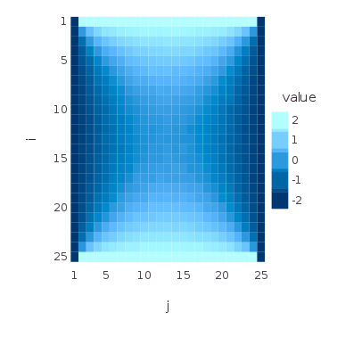
is the exterior boundary of \( {A} \). In this context, the Dirichlet problem consists in finding a function which is harmonic on \( {A} \) and for which the value on \( {\partial\!A} \) is prescribed. This problem is actually a linear algebra problem for which the result below provides a probabilistic expression of the solution, based on the stopping time
\[ \tau_{\partial\!A}:=\inf\{n\geq0:X_n\in\partial\!A\}. \]
In Physics, the quantity \( {f(x)} \) models typically the temperature at location \( {x} \), while the harmonicity of \( {f} \) on \( {A} \) and the boundary condition on \( {\partial\!A} \) express the thermal equilibrium and a thermostatic boundary, respectively.
Theorem 1 (Dirichlet problem) Let \( {\varnothing\neq A\subset\mathbb{Z}^d} \) be finite. Then for any \( {x\in A} \),
\[ \mathbb{P}_x(\tau_{\partial\!A}<\infty)=1. \]
Moreover, for any \( {g:\partial\!A\rightarrow\mathbb{R}} \), the function \( {f:\bar{A}\rightarrow\mathbb{R}} \) defined for any \( {x\in\bar{A}} \) by
\[ f(x)=\mathbb{E}_x(g(X_{\tau_{\partial\!A}})) \]
is the unique solution of the system
\[ \left\{ \begin{array}{rl} f=g &\mbox{on } \partial\!A,\\ \Delta f=0&\mbox{on } A. \end{array} \right. \]
When \( {d=1} \) we recover the function which appears in the gambler ruin problem. Recall that the image of a Markov chain by a function which is harmonic for the generator of the chain is a martingale (discrete Itô formula !), and this explains a posteriori the probabilistic formula for the solution of the Dirichlet problem, thanks to the Doob optional stopping theorem.
The quantity \( {f(x)=\mathbb{E}_x(g(\tau_{\partial\!A}))=\sum_{y\in\partial\!A}g(y)\mathbb{P}_x(\tau_{\partial\!A}=y)} \) is the mean of \( {g} \) for the law \( {\mu_x} \) on \( {\partial\!A} \) called the harmonic measure defined for any \( {y\in\partial\!A} \) by
\[ \mu_x(y):=\mathbb{P}_x(X_{\tau_{\partial\!A}}=y) \]
Proof: The property \( {\mathbb{P}_x(\tau_{\partial\!A}<\infty)=1} \) follows from the Central Limit Theorem or by using conditioning which gives a geometric upper bound for the tail of \( {\tau_{\partial\!A}} \).
Let us check that the proposed function \( {f} \) is a solution. For any \( {x\in\partial\!A} \), we have \( {\tau_{\partial\!A}=0} \) on \( {\{X_0=x\}} \) and thus \( {f=g} \) on \( {\partial\!A} \). Let us show now that \( {\Delta f=0} \) on \( {A} \). We first reduce the problem by linearity to the case \( {g=\mathbf{1}_{\{z\}}} \) with \( {z\in\partial\!A} \). Next, we write, for any \( {y\in\bar{A}} \),
\[ \begin{array}{rcl} f(y) &=&\mathbb{P}_y(X_{\tau_{\partial\!A}}=z)\\ &=&\sum_{n=0}^\infty\mathbb{P}_y(X_n=z,\tau_{\partial\!A}=n)\\ &=&\mathbf{1}_{y=z}+\mathbf{1}_{y\in A}\sum_{n=1}^\infty\sum_{x_1,\ldots,x_{n-1}\in A}P(y,x_1)P(x_1,x_2)\cdots P(x_{n-1},z). \end{array} \]
On the other hand, since \( {f=0} \) on \( {\partial\!A\setminus\{z\}} \) and since \( {\Delta} \) is local, we have, for any \( {x\in A} \),
\[ (P f)(x) =\sum_{y\in\mathbb{Z}^d}P(x,y)f(y) =P(x,z)f(z)+\sum_{y\in A}P(x,y)f(y). \]
As a consequence, for any \( {x\in A} \),
\[ \begin{array}{rcl} (P f)(x) &=&P(x,z)f(z)+\sum_{n=1}^\infty\sum_{y,x_1,\ldots,x_{n-1}\in A} P(x,y)P(y,x_1)\cdots P(x_{n-1},z)\\ &=&P(x,z)f(z)+(f(x)-(\mathbf{1}_{x=z}+P(x,z))), \end{array} \]
which is equal to \( {f(x)} \) since \( {\mathbf{1}_{x=z}=0} \) and \( {f(z)=1} \). Hence \( {Pf=f} \) on \( {A} \), in other words \( {\Delta f=0} \) on \( {A} \).
To establish the uniqueness of the solution, we first reduce the problem by linearity to show that \( {f=0} \) is the unique solution when \( {g=0} \). Next, if \( {f:\bar{A}\rightarrow\mathbb{R}} \) is harmonic on \( {A} \), the interpretation of \( {\Delta f(x)} \) as a difference with the mean on the nearest neighbors allows to show that both the minimum and the maximum of \( {f} \) on \( {\bar{A}} \) are (at least) necessarily achieved on the boundary \( {\partial\!A} \). But since \( {f} \) is vanishes on \( {\partial\!A} \), it follows that \( {f} \) vanishes on \( {\bar{A}} \). ☐
Dirichlet problem and Green function. Here is a generalization of Theorem 1. When \( {h=0} \) we recover Theorem 1.
Theorem 2 (Dirichlet problem and Green function) If \( {\varnothing\neq A\subset\mathbb{Z}^d} \) is finite then for any \( {g:\partial\!A\rightarrow\mathbb{R}} \) and \( {h:A\rightarrow\mathbb{R}} \), the function \( {f:\bar{A}\rightarrow\mathbb{R}} \) defined for any \( {x\in\bar{A}} \) by
\[ f(x)=\mathbb{E}_x\left(g(X_{\tau_{\partial\!A}})+\sum_{n=0}^{\tau_{\partial\!A}-1}h(X_n)\right) \]
is the unique solution of
\[ \left\{ \begin{array}{rl} f=g&\mbox{on } \partial\!A,\\ \Delta f=-h&\mbox{on } A. \end{array} \right. \]
When \( {d=1} \) and \( {h=1} \) then we recover a function which appears in the analysis of the gambler ruin problem.
For any \( {x\in A} \) we have
\[ f(x) =\sum_{y\in\partial\!A}g(y)\mathbb{P}_x(\tau_{\partial\!A}=y)+\sum_{y\in A}h(y)G_A(x,y) \]
where \( {G_A(x,y)} \) is the average number of passages at \( {y} \) starting from \( {x} \) and before escaping from \( {A} \):
\[ G_A(x,y):=\mathbb{E}_x\left\{\sum_{n=0}^{\tau_{\partial\!A}-1}\mathbf{1}_{X_n=y}\right\} =\sum_{n=0}^\infty\mathbb{P}_x(X_n=y,n<\tau_{\partial\!A}). \]
We say that \( {G_A} \) is the Green function of the symmetric nearest neighbors random walk on \( {A} \) killed at the boundary \( {\partial\!A} \). It is the inverse of the restriction \( {-\Delta_A} \) of \( {-\Delta} \) to functions on \( {\bar{A}} \) vanishing on \( {\partial\!A} \):
\[ G_A=-\Delta_A^{-1}. \]
Indeed, when \( {g=0} \) and \( {h=\mathbf{1}_{\{y\}}} \) we get \( {f(x)=G_A(x,y)} \) and thus \( {\Delta_AG_A=-I_A} \).
Proof: Thanks to Theorem 1 it suffices by linearity to check that \( {f(x)=\mathbf{1}_{x\in A}G_A(x,z)} \) is a solution when \( {g=0} \) and \( {h=\mathbf{1}_{\{z\}}} \) with \( {z\in A} \). Now for any \( {x\in A} \),
\[ \begin{array}{rcl} f(x) &=&\mathbf{1}_{\{x=z\}}+\sum_{n=1}^\infty\mathbb{P}_x(X_n=z,n<\tau_{\partial\!A})\\ &=&\mathbf{1}_{\{x=z\}}+\sum_{y:\left|x-y\right|_1=1}\sum_{n=1}^\infty\mathbb{P}(X_n=z,n<\tau_{\partial\!A}\,|\,X_1=y)P(x,y)\\ &=&\mathbf{1}_{\{x=z\}}+\sum_{u:\left|x-y\right|_1=1}f(y)P(x,y) \end{array} \]
thanks to the Markov property. We have \( {f=h+Pf} \) on \( {A} \), in other words \( {\Delta f=-h} \) on \( {A} \). ☐
Beyond the symmetric nearest neighbors random walk. The proofs of Theorem 1 and Theorem 2 remain valid for asymmetric nearest neighbors random walks on \( {\mathbb{Z}^d} \), provided that we replace the generator \( {\Delta} \) of the symmetric nearest neighbors random walk by the generator \( {L:=P-I} \), which is still a local operator: \( {\left|x-y\right|>1\Rightarrow L(x,y)=P(x,y)=0} \). One may even go beyond this framework by adapting the notion of boundary: \( {\{y\not\in A:\exists x\in A, L(x,y)>0\}} \).
Gaussian free field. The Gaussian free field is model of Gaussian random interface for which the covariance matrix is the Green function of the discrete Laplace operator. More precisely, let \( {\varnothing\neq A\subset\mathbb{Z}^d} \) be a finite set. An interface is a height function \( {f:\bar{A}\rightarrow\mathbb{R}} \) which associates to each site \( {x\in\bar{A}} \) a height \( {f(x)} \), also called spin in the context of Statistical Physics. For simplicity, we impose a zero boundary condition: \( {f=0} \) on the boundary \( {\partial\!A} \) of \( {A} \).
Let \( {\mathcal{F}_A} \) be the set of interfaces \( {f} \) on \( {\bar{A}} \) vanishing at the boundary \( {\partial\!A} \), which can be identified with \( {\mathbb{R}^A} \). The energy \( {H_A(f)} \) of the interface \( {f\in\mathcal{F}_A} \) is defined by
\[ H_A(f)=\frac{1}{4d}\sum_{\substack{\{x,y\}\subset\bar{A}\\\left|x-y\right|_1=1}}(f(x)-f(y))^2, \]
where \( {f=0} \) on \( {\partial\!A} \). The flatter is the interface, the smaller is the energy \( {H_A(f)} \). Denoting \( {\left<u,v\right>_A:=\sum_{x\in A}u(x)v(x)} \), we get, for any \( {f\in\mathcal{F}_A} \),
\[ H_A(f) =\frac{1}{4d}\sum_{x\in A}\sum_{\substack{y\in\bar{A}\\\left|x-y\right|_1=1}}(f(x)-f(y))f(x) =\frac{1}{2}\left<-\Delta f,f\right>_A. \]
Since \( {H_A(0)=0} \) and \( {H_A(f)=0} \) give \( {f=0} \), the quadratic form \( {H_A} \) is not singular and we can define the Gaussian law \( {Q_A} \) on \( {\mathcal{F}_A} \) which favors low energies:
\[ Q_A(df)=\frac{1}{Z_A}e^{-H_A(f)}\,df \quad\mbox{where}\quad Z_A:=\int_{\mathcal{F}_A}\!e^{-H_A(f)}\,df. \]
This Gaussian law, called the Gaussian free field, is characterized by its mean \( {m_A:A\rightarrow\mathbb{R}} \) and its covariance matrix \( {C_A:A\times A\rightarrow\mathbb{R}} \), given for any \( {x,y\in A} \) by
\[ m_A(x):=\int\!f_x\,Q_A(df)=0 \]
and
\[ C_A(x,y):=\int\!f_xf_y\,Q_A(df)-m_A(x)m_A(y)=-\Delta_A^{-1}(x,y)=G_A(x,y), \]
where \( {f_x} \) denotes the coordinate map \( {f_x:f\in\mathcal{F}_A\mapsto f(x)\in\mathbb{R}} \).
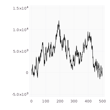
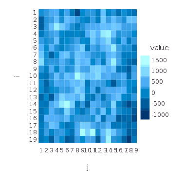
Simulation of the Gaussian free field. The simulation of the Gaussian free field can be done provided that we know how to compute a square root of \( {G_A} \) in the sense of quadratic forms, using for instance a Cholesky factorization or diagonalization. Let us consider the square case:
\[ A=L(0,1)^d\cap\mathbb{Z}^d=\{1,\ldots,L-1\}^d. \]
This gives \( {\bar{A}=\{0,1,\ldots,L\}^d} \). In this case, one can compute the eigenvectors and eigenvalues of \( {\Delta_A} \) and deduce the ones of \( {G_A=-\Delta_A^{-1}} \). In fact, the continuous Laplace operator \( {\Delta} \) on \( {[0,1]^d\in\mathbb{R}^n} \), with Dirichlet boundary conditions, when defined on the Sobolev space \( {\mathrm{H}_0^2([0,1]^d)} \), is a symmetric operator with eigenvectors \( {\{e_n:n\in\{1,2,\ldots\}^d\}} \) and eigenvalues \( {\{\lambda_n:n\in\{1,2,\ldots\}^d\}} \) given by
\[ e_n(t):=2^{d/2}\prod_{i=1}^d\sin(\pi n_i t_i), \quad\mbox{and}\quad \lambda_n:=-\pi^2\left|n\right|_2^2 =-\pi^2(n_1^2+\cdots+n_d^2). \]
Similarly, the discrete Laplace operator \( {\Delta_A} \) with Dirichlet boundary conditions on this \( {A} \) has eigenvectors \( {\{e^L_n:n\in A\}} \) and eigenvalues \( {\{\lambda_n^L:n\in A\}} \) given for any \( {k\in A} \) by
\[ e^L_n(k):=e_n\left(\frac{k}{L}\right) \quad\mbox{and}\quad \lambda_n^L:=-2\,\sum_{i=1}^d \sin^2\left(\frac{\pi n_i}{2L}\right). \]
The vectors \( {e_n^L} \) vanish on the boundary \( {\partial\!A} \). It follows that for any \( {x,y\in A} \),
\[ \Delta_A(x,y)=\sum_{n\in A}\lambda_n^L\left<e^L_n,f_x\right>\left<e^L_n,f_y\right> =\sum_{n\in A}\lambda_n^L e^L_n(x)e^L_n(y) \]
and
\[ G_A(x,y)=-\sum_{n\in A}\left(\lambda_n^L\right)^{-1} e^L_n(x)e^L_n(y). \]
A possible matrix square root \( {\sqrt{G_A}} \) of \( {G_A} \) is given for any \( {x,y\in A} \) by
\[ \sqrt{G_A}(x,y)=-\sum_{n\in A}\left(\lambda_n^L\right)^{-1/2} e^L_n(x)e^L_n(y). \]
Now if \( {Z={(Z_y)}_{y\in A}} \) are independent and identically distributed Gaussian random variables with zero mean and unit variance, seen as a random vector of \( {\mathbb{R}^A} \), then the random vector
\[ \sqrt{G_A}Z = \left(\sum_{y\in A}\sqrt{G_A}(x,y)Z_y\right)_{x\in A} =\left(\sum_{y\in A}\sum_{n\in A}\left(-\lambda_n^L\right)^{-1/2}e_n^L(x)e_n^L(y)Z_y\right)_{x\in A} \]
is distributed according to the Gaussian free field \( {Q_A} \).
Continuous analogue. The scaling limit \( {\varepsilon\mathbb{Z}^d\rightarrow\mathbb{R}^d} \) leads to natural continuous objects (in time and space): the simple random walk becomes the standard Brownian Motion via the Central Limit Theorem, the discrete Laplace operator becomes the Laplace second order differential operator via a Taylor formula, while the discrete Gaussian free field becomes the continuous Gaussian free field (its covariance is the Green function of the Laplace operator). The continuous object are less elementary since their require much more analytic and probabilistic machinery, but in the mean time, they provide differential calculus, a tool which is problematic in discrete settings due in particular to the lack of chain rule.
Further reading.
- James Glimm and Arthur Jaffe. Quantum Physics: A Functional Integral Point of View, mostly chapter 7 "Covariance Operator = Green's Function = Resolvent Kernel = Euclidean Propagator = Fundamental Solution" (great source of inspiration);
- Richard F. Bass. Probabilistic techniques in analysis (very pleasant)
- Scott Scheffield. Gaussian free fields for mathematicians (not so bad, after all)
- Gregory Lawler. Intersections of random walks mostly chapter 1 (old memories from my Master degree memoir!).
Note. The probabilistic approach to the Dirichlet problem goes back at least to Shizuo Kakutani (1911 - 2004), who studied around 1944 the continuous version with Brownian Motion. This post is the English translation of an excerpt from a forthcoming book on stochastic models, written, in French, together with my old friend Florent Malrieu.
#
# load within julia using include("dirichlet.jl")
#
nx, ny = 25, 25
f = zeros(nx,ny)
f[1,:], f[nx,:], f[:,1], f[:,ny] = 2, 2, -2, -2
C = zeros(nx,ny)
N = 5000
#
for x = 1:nx
 for y = 1:ny
  for k = 1:N
   xx = x
   yy = y
   while ((xx > 1) && (xx < nx) && (yy > 1) && (yy < ny))
    b = rand(2)
    if (b[1] < .5)
     if (b[2] < .5)
      xx -= 1
     else
      xx += 1
     end
    elseif (b[2] < .5)
     yy -= 1
    else
     yy += 1
    end
   end # while
   C[x,y] += f[xx,yy]
  end # for k
 end # for y
end # for x
using Compose, Gadfly
draw(PNG("dirichlet.png", 10cm, 10cm), spy(C/N))
#
# load within julia using include("gff.jl")
#
Pkg.add("Gadfly") # produces "INFO: Nothing to be done." if already installed.
Pkg.add("Cairo") # idem.
#Pkg.add("PyPlot") # idem.
using Compose, Gadfly, Cairo # for 2D graphics
#using PyPlot # for 3D graphics (Gadfly does not provide 3D graphics)
#
# dimension 1
#
L = 500
Z = randn(L-1)
lambda = 2*sin(pi*[1:L-1]/(2*L)).^2
evec = sqrt(2)*sin(pi*kron([1:L-1],[1:L-1]')/L)
GFF1 = zeros(L-1)
for x = 1:L-1
    for y = 1:L-1
        for n = 1:L-1
            GFF1[x] += (lambda[n])^(-1/2)*evec[n,x]*evec[n,y]*Z[y]
        end
    end
end
# graphics ith Gadfly
p = plot(x = [1:L-1], y = GFF1,
         Geom.line,
         Guide.xlabel(""),
         Guide.ylabel(""),
         #Guide.title("GFF"),
         Theme(default_color=color("black")))
draw(PNG("gff1.png", 10cm, 10cm), p)
#
# dimension 2
#
L = 20
Z = randn(L-1,L-1)
AUX = kron(ones(L-1)',[1:L-1])
lambda = 2*sin(pi*AUX/(2*L)).^2 + 2*sin(pi*AUX'/(2*L)).^2
evec = zeros(L-1,L-1,L-1,L-1) # n1,n2,k1,k2 : e_n^L(k)
for n1 = 1:L-1
 for n2 = 1:L-1
  AUX = kron(ones(L-1)',[1:L-1])
  evec[n1,n2,:,:] = reshape(2*sin(pi*n1*AUX/L).*sin(pi*n2*AUX'/L),(1,1,L-1,L-1))
 end
end
GFF2 = zeros(L-1,L-1)
for x1 = 1:L-1
 for x2 = 1:L-1
  for y1 = 1:L-1
   for y2 = 1:L-1
    for n1 = 1:L-1
     for n2 = 1:L-1
      aux = (lambda[n1,n2])^(-1/2)
      aux *= evec[n1,n2,x1,x2]
      aux *= evec[n1,n2,y1,y2]
      aux *= Z[y1,y2]
      GFF2[x1,x2] += aux
     end
    end
   end
  end
 end
end
# graphics with PyPlot
#surf(GFF2)
#savefig("gff2.svg")
# graphics with Gadfly
draw(PNG("gff2.png", 10cm, 10cm), spy(GFF2))